A core, emerging problem in nonconvex optimization involves the escape of saddle points. While recent research has shown that gradient descent (GD) generically escapes saddle points asymptotically (see Rong Ge’s and Ben Recht’s blog posts), the critical open problem is one of efficiency— is GD able to move past saddle points quickly, or can it be slowed down significantly? How does the rate of escape scale with the ambient dimensionality? In this post, we describe our recent work with Rong Ge, Praneeth Netrapalli and Sham Kakade, that provides the first provable positive answer to the efficiency question, showing that, rather surprisingly, GD augmented with suitable perturbations escapes saddle points efficiently; indeed, in terms of rate and dimension dependence it is almost as if the saddle points aren’t there!

Perturbing Gradient Descent

We are in the realm of classical gradient descent (GD) — given a function $f:\mathbb{R}^d \to \mathbb{R}$ we aim to minimize the function by moving in the direction of the negative gradient:

where $x_t$ are the iterates and $\eta$ is the step size. GD is well understood theorietically in the case of convex optimization, but the general case of nonconvex optimization has been far less studied. We know that GD converges quickly to the neighborhood of stationary points (points where $\nabla f(x) = 0$) in the nonconvex setting, but these stationary points may be local minima or, unhelpfully, local maxima or saddle points.

Clearly GD will never move away from a stationary point if started there (even a local maximum); thus, to provide general guarantees, it is necessary to modify GD slightly to incorporate some degree of randomness. Two simple methods have been studied in the literature:

1. Intermittent Perturbations: Ge, Huang, Jin and Yuan 2015 considered adding occasional random perturbations to GD, and were able to provide the first polynomial time guarantee for GD to escape saddle points. (See also Rong Ge’s post )

2. Random Initialization: Lee et al. 2016 showed that with only random initialization, GD provably avoids saddle points asymptotically (i.e., as the number of steps goes to infinity). (see also Ben Recht’s post)

Asymptotic — and even polynomial time —results are important for the general theory, but they stop short of explaining the success of gradient-based algorithms in practical nonconvex problems. And they fail to provide reassurance that runs of GD can be trusted — that we won’t find ourselves in a situation in which the learning curve flattens out for an indefinite amount of time, with the user having no way of knowing that the asymptotics have not yet kicked in. Lastly, they fail to provide reassurance that GD has the kind of favorable properties in high dimensions that it is known to have for convex problems.

One reasonable approach to this issue is to consider second-order (Hessian-based) algorithms. Although these algorithms are generally (far) more expensive per iteration than GD, and can be more complicated to implement, they do provide the kind of geometric information around saddle points that allows for efficient escape. Accordingly, a reasonable understanding of Hessian-based algorithms has emerged in the literature, and positive efficiency results have been obtained.

Is GD also efficient? Or is the Hessian necessary for fast escape of saddle points?

A negative result emerges to this first question if one considers the random initialization strategy discussed. Indeed, this approach is provably inefficient in general, taking exponential time to escape saddle points in the worst case (see “On the Necessity of Adding Perturbations” section).

Somewhat surprisingly, it turns out that we obtain a rather different — and positive— result if we consider the perturbation strategy. To be able to state this result, let us be clear on the algorithm that we analyze:

Perturbed gradient descent (PGD)

1. for $~t = 1, 2, \ldots ~$ do
2. $\quad\quad x_{t} \leftarrow x_{t-1} - \eta \nabla f (x_{t-1})$
3. $\quad\quad$ if $~$perturbation condition holds$~$ then
4. $\quad\quad\quad\quad x_t \leftarrow x_t + \xi_t$

Here the perturbation $\xi_t$ is sampled uniformly from a ball centered at zero with a suitably small radius, and is added to the iterate when the gradient is suitably small. These particular choices are made for analytic convenience; we do not believe that uniform noise is necessary. nor do we believe it essential that noise be added only when the gradient is small.

Strict-Saddle and Second-order Stationary Points

We define saddle points in this post to include both classical saddle points as well as local maxima. They are stationary points which are locally maximized along at least one direction. Saddle points and local minima can be categorized according to the minimum eigenvalue of Hessian:

We further call the saddle points in the last category, where $\lambda_{\min}(\nabla^2 f(x)) < 0$, strict saddle points.

While non-strict saddle points can be flat in the valley, strict saddle points require that there is at least one direction along which the curvature is strictly negative. The presence of such a direction gives a gradient-based algorithm the possibility of escaping the saddle point. In general, distinguishing local minima and non-strict saddle points is NP-hard; therefore, we — and previous authors — focus on escaping strict saddle points.

Formally, we make the following two standard assumptions regarding smoothness.

Assumption 1: $f$ is $\ell$-gradient-Lipschitz, i.e.
$\quad\quad\quad\quad \forall x_1, x_2, |\nabla f(x_1) - \nabla f(x_2)| \le \ell |x_1 - x_2|$.
$~$
Assumption 2: $f$ is $\rho$-Hessian-Lipschitz, i.e.
$\quad\quad\quad\quad \forall x_1, x_2$, $|\nabla^2 f(x_1) - \nabla^2 f(x_2)| \le \rho |x_1 - x_2|$.

Similarly to classical theory, which studies convergence to a first-order stationary point, $\nabla f(x) = 0$, by bounding the number of iterations to find a $\epsilon$-first-order stationary point, $|\nabla f(x)| \le \epsilon$, we formulate the speed of escape of strict saddle points and the ensuing convergence to a second-order stationary point, $\nabla f(x) = 0, \lambda_{\min}(\nabla^2 f(x)) \ge 0$, with an $\epsilon$-version of the definition:

Definition: A point $x$ is an $\epsilon$-second-order stationary point if:
$\quad\quad\quad\quad |f(x)|\le \epsilon$, and $\lambda_{\min}(\nabla^2 f(x)) \ge -\sqrt{\rho \epsilon}$.

In this definition, $\rho$ is the Hessian Lipschitz constant introduced above. This scaling follows the convention of Nesterov and Polyak 2006.

Applications

In a wide range of practical nonconvex problems it has been proved that all saddle points are strict— such problems include, but not are limited to, principal components analysis, canonical correlation analysis, orthogonal tensor decomposition, phase retrieval, dictionary learning, matrix sensing, matrix completion, and other nonconvex low-rank problems.

Furthermore, in all of these nonconvex problems, it also turns out that all local minima are global minima. Thus, in these cases, any general efficient algorithm for finding $\epsilon$-second-order stationary points immediately becomes an efficient algorithm for solving those nonconvex problem with global guarantees.

Escaping Saddle Point with Negligible Overhead

In the classical case of first-order stationary points, GD is known to have very favorable theoretical properties:

Theorem (Nesterov 1998): If Assumption 1 holds, then GD, with $\eta = 1/\ell$, finds an $\epsilon$-first-order stationary point in $2\ell (f(x_0) - f^\star)/\epsilon^2$ iterations.

In this theorem, $x_0$ is the initial point and $f^\star$ is the function value of the global minimum. The theorem says for that any gradient-Lipschitz function, a stationary point can be found by GD in $O(1/\epsilon^2)$ steps, with no explicit dependence on $d$. This is called “dimension-free optimization” in the literature; of course the cost of a gradient computation is $O(d)$, and thus the overall runtime of GD scales as $O(d)$. The linear scaling in $d$ is especially important for modern high-dimensional nonconvex problems such as deep learning.

We now wish to address the corresponding problem for second-order stationary points. What is the best we can hope for? Can we also achieve

1. A dimension-free number of iterations;
2. An $O(1/\epsilon^2)$ convergence rate;
3. The same dependence on $\ell$ and $(f(x_0) - f^\star)$ as in (Nesterov 1998)?

Rather surprisingly, the answer is Yes to all three questions (up to small log factors).

Main Theorem: If Assumptions 1 and 2 hold, then PGD, with $\eta = O(1/\ell)$, finds an $\epsilon$-second-order stationary point in $\tilde{O}(\ell (f(x_0) - f^\star)/\epsilon^2)$ iterations with high probability.

Here $\tilde{O}(\cdot)$ hides only logarithmic factors; indeed, the dimension dependence in our result is only $\log^4(d)$. The theorem thus asserts that a perturbed form of GD, under an additional Hessian-Lipschitz condition, converges to a second-order-stationary point in almost the same time required for GD to converge to a first-order-stationary point. In this sense, we claim that PGD can escape strict saddle points almost for free.

We turn to a discussion of some of the intuitions underlying these results.

Why do polylog(d) iterations suffice?

Our strict-saddle assumption means that there is only, in the worst case, one direction in $d$ dimensions along which we can escape. A naive search for the descent direction intuitively should take at least $\text{poly}(d)$ iterations, so why should only $\text{polylog}(d)$ suffice?

Consider a simple case in which we assume that the function is quadratic in the neighborhood of the saddle point. That is, let the objective function be $f(x) = x^\top H x$, a saddle point at zero, with constant Hessian $H = \text{diag}(-1, 1, \cdots, 1)$. In this case, only the first direction is an escape direction (with negative eigenvalue $-1$).

It is straightforward to work out the general form of the iterates in this case:

Assume that we start at the saddle point at zero, then add a perturbation so that $x_0$ is sampled uniformly from a ball $\mathcal{B}_0(1)$ centered at zero with radius one. The decrease in the function value can be expressed as:

Set the step size to be $1/2$, let $\lambda_i$ denote the $i$-th eigenvalue of the Hessian $H$ and let $\alpha_i = e_i^\top x_0$ denote the component in the $i$th direction of the initial point $x_0$. We have $\sum_{i=1}^d \alpha_i^2 = | x_0|^2 = 1$, thus:

A simple probability argument shows that sampling uniformly in $\mathcal{B}_0(1)$ will result in at least a $\Omega(1/d)$ component in the first direction with high probability. That is, $\alpha^2_1 = \Omega(1/d)$. Substituting $\alpha_1$ in the above equation, we see that it takes at most $O(\log d)$ steps for the function value to decrease by a constant amount.

Pancake-shape stuck region for general Hessian

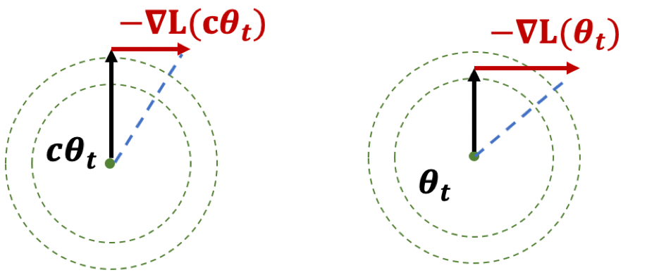
We can conclude that for the case of a constant Hessian, only when the perturbation $x_0$ lands in the set $\{x | ~ |e_1^\top x|^2 \le O(1/d)\}$ $\cap \mathcal{B}_0 (1)$, can we take a very long time to escape the saddle point. We call this set the stuck region; in this case it is a flat disk. In general, when the Hessian is no longer constant, the stuck region becomes a non-flat pancake, depicted as a green object in the left graph. In general this region will not have an analytic expression.

Earlier attempts to analyze the dynamics around saddle points tried to the approximate stuck region by a flat set. This results in a requirement of an extremely small step size and a correspondingly very large runtime complexity. Our sharp rate depends on a key observation — although we don’t know the shape of the stuck region, we know it is very thin.

In order to characterize the “thinness” of this pancake, we studied pairs of hypothetical perturbation points $w, u$ separated by $O(1/\sqrt{d})$ along an escaping direction. We claim that if we run GD starting at $w$ and $u$, at least one of the resulting trajectories will escape the saddle point very quickly. This implies that the thickness of the stuck region can be at most $O(1/\sqrt{d})$, so a random perturbation has very little chance to land in the stuck region.

On the Necessity of Adding Perturbations

We have discussed two possible ways to modify the standard gradient descent algorithm, the first by adding intermittent perturbations, and the second by relying on random initialization. Although the latter exhibits asymptotic convergence, it does not yield efficient convergence in general; in recent joint work with Simon Du, Jason Lee, Barnabas Poczos, and Aarti Singh, we have shown that even with fairly natural random initialization schemes and non-pathological functions, GD with only random initialization can be significantly slowed by saddle points, taking exponential time to escape. The behavior of PGD is strikingingly different — it can generically escape saddle points in polynomial time.

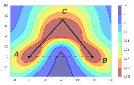
To establish this result, we considered random initializations from a very general class including Gaussians and uniform distributions over the hypercube, and we constructed a smooth objective function that satisfies both Assumptions 1 and 2. This function is constructed such that, even with random initialization, with high probability both GD and PGD have to travel sequentially in the vicinity of $d$ strict saddle points before reaching a local minimum. All strict saddle points have only one direction of escape. (See the left graph for the case of $d=2$).

When GD travels in the vicinity of a sequence of saddle points, it can get closer and closer to the later saddle points, and thereby take longer and longer to escape. Indeed, the time to escape the $i$th saddle point scales as $e^{i}$. On the other hand, PGD is always able to escape any saddle point in a small number of steps independent of the history. This phenomenon is confirmed by our experiments; see, for example, an experiment with $d=10$ in the right graph.

Conclusion

In this post, we have shown that a perturbed form of gradient descent can converge to a second-order-stationary point at almost the same rate as standard gradient descent converges to a first-order-stationary point. This implies that Hessian information is not necessary for to escape saddle points efficiently, and helps to explain why basic gradient-based algorithms such as GD (and SGD) work surprisingly well in the nonconvex setting. This new line of sharp convergence results can be directly applied to nonconvex problem such as matrix sensing/completion to establish efficient global convergence rates.

There are of course still many open problems in general nonconvex optimization. To name a few: will adding momentum improve the convergence rate to a second-order stationary point? What type of local minima are tractable and are there useful structural assumptions that we can impose on local minima so as to avoid local minima efficiently? We are making slow but steady progress on nonconvex optimization, and there is the hope that at some point we will transition from “black art” to “science”.

Unsupervised learning, as the name suggests, is the science of learning from unlabeled data. A look at the wikipedia page shows that this term has many interpretations:

(Task A)Learning a distribution from samples. (Examples: gaussian mixtures, topic models, variational autoencoders,..)

(Task B)Understanding latent structure in the data. This is not the same as (a); for example principal component analysis, clustering, manifold learning etc. identify latent structure but don’t learn a distribution per se.

(Task C)Feature Learning. Learn a mapping from datapoint $\rightarrow$ feature vector such that classification tasks are easier to carry out on feature vectors rather than datapoints. For example, unsupervised feature learning could help lower the amount of labeled samples needed for learning a classifier, or be useful for domain adaptation.

Task B is often a subcase of Task C, as the intended user of “structure found in data” are humans (scientists) who pour over the representation of data to gain some intuition about its properties, and these “properties” can be often phrased as a classification task.

This post explains the relationship between Tasks A and C, and why they get mixed up in students’ mind. We hope there is also some food for thought here for experts, namely, our discussion about the fragility of the usual “perplexity” definition of unsupervised learning. It explains why Task A doesn’t in practice lead to good enough solution for Task C. For example, it has been believed for many years that for deep learning, unsupervised pretraining should help supervised training, but this has been hard to show in practice.

The common theme: high level representations.

If $x$ is a datapoint, each of these methods seeks to map it to a new “high level” representation $h$ that captures its “essence.” This is why it helps to have access to $h$ when performing machine learning tasks on $x$ (e.g. classification). The difficulty of course is that “high-level representation” is not uniquely defined. For example, $x$ may be an image, and $h$ may contain the information that it contains a person and a dog. But another $h$ may say that it shows a poodle and a person wearing pyjamas standing on the beach. This nonuniqueness seems inherent.

Unsupervised learning tries to learn high-level representation using unlabeled data. Each method make an implicit assumption about how the hidden $h$ relates to the visible $x$. For example, in k-means clustering the hidden $h$ consists of labeling the datapoint with the index of the cluster it belongs to. Clearly, such a simple clustering-based representation has rather limited expressive power since it groups datapoints into disjoint classes: this limits its application for complicated settings. For example, if one clusters images according to the labels “human”, “animal” “plant” etc., then which cluster should contain an image showing a man and a dog standing in front of a tree?

The search for a descriptive language for talking about the possible relationships of representations and data leads us naturally to Bayesian models. (Note that these are viewed with some skepticism in machine learning theory – compared to assumptionless models like PAC learning, online learning, etc. – but we do not know of another suitable vocabulary in this setting.)

A Bayesian view

Bayesian approaches capture the relationship between the “high level” representation $h$ and the datapoint $x$ by postulating a joint distribution $p_{\theta}(x, h)$ of the data $x$ and representation $h$, such that $p_{\theta}(h)$ and the posterior $p_{\theta}(x \mid h)$ have a simple form as a function of the parameters $\theta$. These are also called latent variable probabilistic models, since $h$ is a latent (hidden) variable.

The standard goal in distribution learning is to find the $\theta$ that “best explains” the data (what we called Task (A)) above). This is formalized using maximum-likelihood estimation going back to Fisher (~1910-1920): find the $\theta$ that maximizes the log probability of the training data. Mathematically, indexing the samples with $t$, we can write this as

where

(Note that $\sum_{t} \log p_{\theta}(x_t)$ is also the empirical estimate of the cross-entropy $E_{x}[\log p_{\theta}(x)]$ of the distribution $p_{\theta}$, where $x$ is distributed according to $p^*$, the true distribution of the data. Thus the above method looks for the distribution with best cross-entropy on the empirical data, which is also log of the perplexity of $p_{\theta}$.)

In the limit of $t \to ∞$, this estimator is consistent (converges in probability to the ground-truth value) and efficient (has lowest asymptotic mean-square-error among all consistent estimators). See the Wikipedia page. (Aside: maximum likelihood estimation is often NP-hard, which is one of the reasons for the renaissance of the method-of-moments and tensor decomposition algorithms in learning latent variable models, which Rong wrote about some time ago.)

Toward task C: Representations arise from the posterior distribution

Simply learning the distribution $p_{\theta}(x, h)$ does not yield a representation per se. To get a distribution of $x$, we need access to the posterior $p_{\theta}(h \mid x)$: then a sample from this posterior can be used as a “representation” of a data-point $x$. (Aside: Sometimes, in settings when $p_{\theta}(h \mid x)$ has a simple description, this description can be viewed as the representation of $x$.)

Thus solving Task C requires learning distribution parameters $\theta$ and figuring out how to efficiently sample from the posterior distribution.

Note that the sampling problems for the posterior can be #-P hard for very simple families. The reason is that by Bayes law, $p_{\theta}(h \mid x) = \frac{p_{\theta}(h) p_{\theta}(x \mid h)}{p_{\theta}(x)}$. Even if the numerator is easy to calculate, as is the case for simple families, the $p_{\theta}(x)$ involves a big summation (or integral) and is often hard to calculate.

Note that the max-likelihood parameter estimation (Task A) and approximating the posterior distributions $p(h \mid x)$ (Task C) can have radically different complexities: Sometimes A is easy but C is NP-hard (example: topic modeling with “nice” topic-word matrices, but short documents, see also Bresler 2015); or vice versa (example: topic modeling with long documents, but worst-case chosen topic matrices Arora et al. 2011)

Of course, one may hope (as usual) that computational complexity is a worst-case notion and may not apply in practice. But there is a bigger issue with this setup, having to do with accuracy.

Why the above reasoning is fragile: Need for high accuracy

The above description assumes that the parametric model $p_{\theta}(x, h)$ for the data was exact whereas one imagines it is only approximate (i.e., suffers from modeling error). Furthermore, computational difficulties may restrict us to use approximately correct inference even if the model were exact. So in practice, we may only have an approximation $q(h|x)$ to the posterior distribution $p_{\theta}(h \mid x)$. (Below we describe a popular methods to compute such approximations.)

How good of an approximation to the true posterior do we need?

Recall, we are trying to answer this question through the lens of Task C, solving some classification task. We take the following point of view:

For $t=1, 2,\ldots,$ nature picked some $(h_t, x_t)$ from the joint distribution and presented us $x_t$. The true label $y_t$ of $x_t$ is $\mathcal{C}(h_t)$ where $\mathcal{C}$ is an unknown classifier. Our goal is classify according to these labels.

To simplify notation, assume the output of $\mathcal{C}$ is binary. If we wish to use $q(h \mid x)$ as a surrogate for the true posterior $p_{\theta}(h \mid x)$, we need to have $\Pr_{x_t, h_t \sim q(\cdot \mid x_t)} [\mathcal{C}(h_t) \neq y_t]$ is small as well.

How close must $q(h \mid x)$ and $p(h \mid x)$ be to let us conclude this? We will use KL divergence as “distance” between the distributions, for reasons that will become apparent in the following section. We claim the following:

CLAIM: The probability of obtaining different answers on classification tasks done using the ground truth $h$ versus the representations obtained using $q(h_t \mid x_t)$ is less than $\epsilon$ if $KL(q(h_t \mid x_t) \parallel p(h_t \mid x_t)) \leq 2\epsilon^2.$

Here’s a proof sketch. The natural distance these two distributions $q(h \mid x)$ and $p(h \mid x)$ with respect to accuracy of classification tasks is total variation (TV) distance. Indeed, if the TV distance between $q(h\mid x)$ and $p(h \mid x)$ is bounded by $\epsilon$, this implies that for any event $\Omega$,

The CLAIM now follows by instantiating this with the event $\Omega = $ “Classifier $\mathcal{C}$ outputs a different answer from $y_t$ given representation $h_t$ for input $x_t$”, and relating TV distance to KL divergence using Pinsker’s inequality, which gives

as we needed. This observation explains why solving Task A in practice does not automatically lead to very useful representations for classification tasks (Task C): the posterior distribution has to be learnt extremely accurately, which probably didn’t happen (either due to model mismatch or computational complexity).

The link between Tasks A and C: variational methods

As noted, distribution learning (Task A) via cross-entropy/maximum-likelihood fitting, and representation learning (Task C) via sampling the posterior are fairly distinct. Why do students often conflate the two? Because in practice the most frequent way to solve Task A does implicitly compute posteriors and thus also solves Task C.

The generic way to learn latent variable models involves variational methods, which can be viewed as a generalization of the famous EM algorithm (Dempster et al. 1977).

Variational methods maintain at all times a proposed distribution $q(h | x)$ (called variational distribution). The methods rely on the observation that for every such $q(h \mid x)$ the following lower bound holds \begin{equation} \log p(x) \geq E_{q(h \mid x)} \log p(x,h) + H(q(h\mid x)) \qquad (2). \end{equation} where $H$ denotes Shannon entropy (or differential entropy, depending on whether $x$ is discrete or continuous). The RHS above is often called the ELBO bound (ELBO = evidence-based lower bound). This inequality follows from a bit of algebra using non-negativity of KL divergence, applied to distributions $q(h \mid x)$ and $p(h\mid x)$. More concretely, the chain of inequalities is as follows,

Furthermore, equality is achieved if $q(h\mid x) = p(h\mid x)$. (This can be viewed as some kind of “duality” theorem for distributions, and dates all the way back to Gibbs. )

Algorithmically observation (2) is used by foregoing solving the maximum-likelihood optimization (1), and solving instead

Since the variables are naturally divided into two blocks: the model parameters $\theta$, and the variational distributions $q(h_t\mid x_t)$, a natural way to optimize the above is to alternate optimizing over each group, while keeping the other fixed. (This meta-algorithm is often called variational EM for obvious reasons.)

Of course, optimizing over all possible distributions $q$ is an ill-defined problem, so $q$ is constrained to lie in some parametric family (e.g., “ standard Gaussian transformed by depth $4$ neural nets of certain size and architecture”) such the above objective can be easily evaluated at least (typically it has a closed-form expression).

Clearly if the parametric family of distributions is expressive enough, and the (non-convex) optimization problem doesn’t get stuck in bad local minima, then variational EM algorithm will give us not only values of the parameters $\theta$ which are close to the ground-truth ones, but also variational distributions $q(h\mid x)$ which accurately track $p(h\mid x)$. But as we saw above, this accuracy would need to be very high to get meaningful representations.

Next Post

In the next post, we will describe our recent work further clarifying this issue of representation learning via a Bayesian viewpoint.

This post is about our new paper, which presents empirical evidence that current GANs (Generative Adversarial Nets) are quite far from learning the target distribution. Previous posts had introduced GANs and described new theoretical analysis of GANs from our ICML17 paper. One notable implication of our theoretical analysis was that when the discriminator size is bounded, then GANs training could appear to succeed (i.e., training objective reaches its optimum value) even if the generated distribution is discrete and has very low support —-in other words, the training objective is unable to prevent even extreme mode collapse.

That paper led us (especially Sanjeev) into spirited discussions with colleagues, who wondered if this is just a theoretical result about potential misbehavior rather than a prediction about real-life training. After all, we’ve all seen the great pictures that GANs produce in real life, right? (Note that the theoretical result only describes a possible near-equilibrium that can arise with a certain mix of hyperparameters, and conceivably real-life training avoids that by suitable hyperparameter tuning.)

Our new empirical paper Do GANs actually learn the distribution? An empirical study puts the issue to the test. We present empirical evidence that well-known GANs approaches do end up learning distributions of fairly low support, and thus presumably are not learning the target distribution.

Let’s start by imagining how large the support must be for the target distribution. For example, if the distribution is the set of all possible images of human faces (real or imagined), then these must involve all combinations of hair color/style, facial features, complexion, expression, pose, lighting, race, etc., and thus the possible set of images of faces that humans will consider to be distinct approaches infinity. (After all, there are billions of distinct people living on earth right now.) GANs are trying to learn this full distribution using a finite sample of images, say CelebA which has $200,000$ images of celebrity faces.

Thus a simple sanity check for whether a GAN has truly come close to learning this distribution is to estimate how many “distinct” images it can produce. At first glance, such an estimation seems very difficult. After all, automated/heuristic measures of image similarity can be easily fooled, and we humans surely don’t have enough time to go through millions or billions of images, right?

Luckily, a crude estimate is possible using the simple birthday paradox, a staple of undergrad discrete math.

Birthday paradox test for size of the support

Imagine for argument’s sake that the human race were limited to a genetic diversity of a million —nature’s laws only allow this many distinct humans. How would this hard limit manifest itself in our day to day life? The birthday paradox says that if we take a random sample of a thousand people —note that most of us get to know this many people easily in our lifetimes—we’d see many doppelgangers. Of course, in practice the only doppelgangers we encounter happen to be identical twins.

Formally, the birthday paradox says that if a discrete distribution has support $N$, then a random sample of size about $\sqrt{N}$ would be quite likely to contain a duplicate. (The name comes from its implication that if you put $23 \approx \sqrt{365}$ random people in a room, the chance that two of them have the same birthday is about $1/2$.)

In the GAN setting, the distribution is continuous, not discrete. Thus our proposed birthday paradox test for GANs is as follows.

(a) Pick a sample of size $s$ from the generated distribution. (b) Use an automated measure of image similarity to flag the $20$ (say) most similar pairs in the sample. (c) Visually inspect the flagged pairs and check for images that a human would consider near-duplicates. (d) Repeat.

If this test reveals that samples of size $s$ have duplicate images with good probability, then suspect that the distribution has support size about $s^2$.

Note that the test is not definitive, because the distribution could assign say a probability $10\%$ to a single image, and be uniform on a huge number of other images. Then the test would be quite likely to find a duplicate even with $20$ samples, even though the true support size is huge. But such nonuniformity (a lot of probability being assigned to a few images) is the only failure mode of the birthday paradox test calculation, and such nonuniformity would itself be considered a failure mode of GANs training. The CIFAR-10 samples below show that such nonuniformality can be severe in practice, where the generator tends to generate a fixed image of automobile very likely. On CIFAR-10, this failure mode is also observed in classes of frogs and cats.

Experimental results.

Our test was done using two datasets, CelebA (faces) and CIFAR-10.

For faces, we found Euclidean distance in pixel space works well as a heuristic similarity measure, probably because the samples are centered and aligned. For CIFAR-10, we pre-train a discriminative Convolutional Neural Net for the full classification problem, and use the top layer representation as an embedding of the image. Heuristic similarity is then measured as the Euclidean distance in the embedding space. Possibly these similarity measures are crude, but note that improving them can only lower our estimate of the support size of the distribution, since a better similarity measure can only increase the number of duplicates found. Thus our estimates below should be considered as upper bounds on the support size of the distribution.

Results on CelebA dataset

We tested the following methods, doing the birthday paradox test with Euclidean distance in pixel space as the heuristic similarity measure.

• DCGAN —unconditional as described in Goodfellow et al. 2014 and Radford et al. 2015
• MIX+GAN protocol introduced in Arora et al., specifically, MIX+DCGAN with $3$ mixture components.
• Adversarily Learned Inference (ALI) (or equivalently BiGANs). (ALI is probabilistic version of BiGANs, but their architectures are equivalent. So we only tested ALI in our experiments.)

We find that with probability $\geq50\%$, a batch of about $400$ samples contains at least one pair of duplicates for both DCGAN and MIX+DCGAN. The figure below give examples duplicates and their nearest neighbors samples (that we could fine) in training set. These results suggest that the support size of the distribution is less than $400^2\approx160000$, which is actually lower than the diversity of the training set, but this distribution is not just memorizing the training set.

ALI (or BiGANs) appear to be somewhat more diverse, in that collisions appear with $50\%$ probability only with a batch size of $1000$, implying a support size of a million. This is $5$x the training set, but still much smaller than the diversity one would expect among human faces (After all doppelgangers don’t appear in samples of a few thousand people in real life.) For fair comparison, we set the discriminator of ALI (or BiGANs) to be roughly the same in size as that of the DCGAN model, since the results below suggests that the discriminator size has a strong effect on diversity of the learnt distribution.) Nevertheless, these tests do support the suggestion that the bidirectional structure prevents some of the mode collapses observed in usual GANs.

Diversity vs Discriminator Size

The analysis of Arora et al. suggested that the support size could be as low as near-linear in the capacity of the discriminator; in other words, there is a near-equilibrium in which a distribution of such a small support could suffice to fool the best discriminator. So it is worth investigating whether training in real life allows generator nets to exploit this “loophole” in the training that we now know is in principle available to them.

We built DCGANs with increasingly larger discriminators while fixing the other hyper-parameters. The discriminator used here is a 5-layer Convolutional Neural Network such that the number of output channels of each layer is $1\times,2\times,4\times,8\times\textit{dim}$ where $dim$ is chosen to be $16,32,48,64,80,96,112,128$. Thus the discriminator size should be proportional to $dim^2$. The figure below suggests that in this simple setup the diversity of the learnt distribution does indeed grow near-linearly with the discriminator size. (Note the diversity is seen to plateau, possibly because one needs to change other parameters like depth to meaningfully add more capacity to the discriminator.)

Results for CIFAR-10

On CIFAR-10, as mentioned earlier, we use a heuristic image similarity computed with convolutional neural net with 3 convolutional layers, 2 fully-connected layer and a 10-class soft-max output pretrained with a multi-class classification objective. Specifically, the top layer features are viewed as embeddings for similarity test using Euclidean distance. We found that this heuristic similarity test quickly becomes useless if the samples display noise artifacts, and thus was effective only on the very best GANs that generate the most real-looking images. For CIFAR-10 this led us to Stacked GAN, currently believed to be the best generative model on CIFAR-10 (Inception Score $8.59$). Since this model is trained by conditioning on class label, we measure its diversity within each class separately.

The training set for each class has $10k$ images, but since the generator is allowed to learn from all classes, presumably it can mix and match (especially background, lighting, landscape etc.) between classes and learn a fairly rich set of images.

Now we list the batch sizes needed for duplicates to appear.

As before, we show duplicate samples as well as the nearest neighbor to the samples in training set (identified by using heuristic similarity measure to flag possibilities and confirming visually).

We find that the closest image is quite different from the duplicate detected, which suggests the issue with GANs is indeed lack of diversity (low support size) instead of memorizing training set. (See the paper for more examples.)

Note that by and large the diversity of the learnt distribution is higher than that of the training set, but still not as high as one would expect in terms of all possible combinations.

Birthday paradox test for VAEs

Given these findings, it is natural to wonder about the diversity of distributions learned using earlier methods such as Variational Auto-Encoders (VAEs). Instead of using feedback from the discriminator, these methods train the generator net using feedback from an approximate perplexity calculation. Thus the analysis of Arora et al. does not apply as is to such methods and it is conceivable they exhibit higher diversity. However, we found the birthday paradox test difficult to run since samples from a VAE trained on CelebA were not realistic or sharp enough for a human to definitively conclude whether or not two images were almost the same. The figure above shows examples of collision candidates found in batches of 400 samples; clearly some indicative parts (hair, eyes, mouth, etc.) are quite blurry in VAE samples.

Conclusions

Our new birthday paradox test seems to suggest that some well-regarded GANs are currently learning distributions that with rather low support (i.e., suffer mode collapse). The possibility of such a scenario was anticipated in the theoretical analysis of (Arora et al.) reported in an earlier post.

This combination of theory and empirics raises the open problem of how to change the GANs training to avoid such mode collapse. Possibly ALI/BiGANs point to the right direction, since they exhibit somewhat better diversity in our experiments. One should also try tuning of hyperparameter/architecture in current methods now that the birthday paradox test gives a concrete way to quantify mode collapse.

Finally, we should consider the possibility that the best use of GANs and related techniques could be feature learning or some other goal, as opposed to distribution learning. This needs further theoretical and empirical exploration.

Deep learning holds many mysteries for theory, as we have discussed on this blog. Lately many ML theorists have become interested in the generalization mystery: why do trained deep nets perform well on previously unseen data, even though they have way more free parameters than the number of datapoints (the classic “overfitting” regime)? Zhang et al.’s paper Understanding Deep Learning requires Rethinking Generalization played some role in bringing attention to this challenge. Their main experimental finding is that if you take a classic convnet architecture, say Alexnet, and train it on images with random labels, then you can still achieve very high accuracy on the training data. (Furthermore, usual regularization strategies, which are believed to promote better generalization, do not help much.) Needless to say, the trained net is subsequently unable to predict the (random) labels of still-unseen images, which means it doesn’t generalize. The paper notes that the ability to fit a classifier to data with random labels is also a traditional measure in machine learning called Rademacher complexity (which we will discuss shortly) and thus Rademacher complexity gives no meaningful bounds on sample complexity. I found this paper entertainingly written and recommend reading it, despite having given away the punchline. Congratulations to the authors for winning best paper at ICLR 2017.

But I would be remiss if I didn’t report that at the Simons Institute Semester on theoretical ML in spring 2017 generalization theory experts expressed unhappiness about this paper, and especially its title. They felt that similar issues had been extensively studied in context of simpler models such as kernel SVMs (which, to be fair, is clearly mentioned in the paper). It is trivial to design SVM architectures with high Rademacher complexity which nevertheless train and generalize well on real-life data. Furthermore, theory was developed to explain this generalization behavior (and also for related models like boosting). On a related note, several earlier papers of Behnam Neyshabur and coauthors (see this paper and for a full account, Behnam’s thesis) had made points fairly similar to Zhang et al. pertaining to deep nets.

But regardless of such complaints, we should be happy about the attention brought by Zhang et al.’s paper to a core theory challenge. Indeed, the passionate discussants at the Simons semester themselves banded up in subgroups to address this challenge: these resulted in papers by Dzigaite and Roy, then Bartlett, Foster, and Telgarsky and finally Neyshabur, Bhojapalli, MacAallester, Srebro. (The latter two were presented at NIPS’17 this week.)

Before surveying these results let me start by suggesting that some of the controversy over the title of Zhang et al.’s paper stems from some basic confusion about whether or not current generalization theory is prescriptive or merely descriptive. These confusions arise from the standard treatment of generalization theory in courses and textbooks, as I discovered while teaching the recent developments in my graduate seminar.

Prescriptive versus descriptive theory

To illustrate the difference, consider a patient who says to his doctor: “Doctor, I wake up often at night and am tired all day.”

Doctor 1 (without any physical examination): “Oh, you have sleep disorder.”

I call such a diagnosis descriptive, since it only attaches a label to the patient’s problem, without giving any insight into how to solve the problem. Contrast with:

Doctor 2 (after careful physical examination): “A growth in your sinus is causing sleep apnea. Removing it will resolve your problems.”

Such a diagnosis is prescriptive.

Generalization theory: descriptive or prescriptive?

Generalization theory notions such as VC dimension, Rademacher complexity, and PAC-Bayes bound, consist of attaching a descriptive label to the basic phenomenon of lack of generalization. They are hard to compute for today’s complicated ML models, let alone to use as a guide in designing learning systems.

Recall what it means for a hypothesis/classifier $h$ to not generalize. Assume the training data consists of a sample $S = {(x_1, y_1), (x_2, y_2),\ldots, (x_m, y_m)}$ of $m$ examples from some distribution ${\mathcal D}$. A loss function $\ell$ describes how well hypothesis $h$ classifies a datapoint: the loss $\ell(h, (x, y))$ is high if the hypothesis didn’t come close to producing the label $y$ on $x$ and low if it came close. (To give an example, the regression loss is $(h(x) -y)^2$.) Now let us denote by $\Delta_S(h)$ the average loss on samplepoints in $S$, and by $\Delta_{\mathcal D}(h)$ the expected loss on samples from distribution ${\mathcal D}$. Training generalizes if the hypothesis $h$ that minimises $\Delta_S(h)$ for a random sample $S$ also achieves very similarly low loss $\Delta_{\mathcal D}(h)$ on the full distribution. When this fails to happen, we have:

Lack of generalization: $\Delta_S(h) \ll \Delta_{\mathcal D}(h) \qquad (1). $

In practice, lack of generalization is detected by taking a second sample (“held out set”) $S_2$ of size $m$ from ${\mathcal D}$. By concentration bounds expected loss of $h$ on this second sample closely approximates $\Delta_{\mathcal D}(h)$, allowing us to conclude

Generalization Theory: Descriptive Parts

Let’s discuss Rademacher complexity, which I will simplify a bit for this discussion. (See also scribe notes of my lecture.) For convenience assume in this discussion that labels and loss are $0,1$, and assume that the badly generalizing $h$ predicts perfectly on the training sample $S$ and is completely wrong on the heldout set $S_2$, meaning

$\Delta_S(h) - \Delta_{S_2}(h) \approx - 1 \qquad (3)$

Rademacher complexity concerns the following thought experiment. Take a single sample of size $2m$ from $\mathcal{D}$, split it into two and call the first half $S$ and the second $S_2$. Flip the labels of points in $S_2$. Now try to find a classifier $C$ that best describes this new sample, meaning one that minimizes $\Delta_S(h) + 1- \Delta_{S_2}(h)$. This expression follows since flipping the label of a point turns good classification into bad and vice versa, and thus the loss function for $S_2$ is $1$ minus the old loss. We say the class of classifiers has high Rademacher complexity if with high probability this quantity is small, say close to $0$.

But a glance at (3) shows that it implies high Rademacher complexity: $S, S_2$ were random samples of size $m$ from $\mathcal{D}$, so their combined size is $2m$, and when generalization failed we succeeded in finding a hypothesis $h$ for which $\Delta_S(h) + 1- \Delta_{S_2}(h)$ is very small.

In other words, returning to our medical analogy, the doctor only had to hear “Generalization didn’t happen” to pipe up with: “Rademacher complexity is high.” This is why I call this result descriptive.

The VC dimension bound is similarly descriptive. VC dimension is defined to be at least $k +1$ if there exists a set of size $k$ such that the following is true. If we look at all possible classifiers in the class, and the sequence of labels each gives to the $k$ datapoints in the sample, then we can find all possible $2^{k}$ sequences of $0$’s and $1$’s.

If generalization does not happen as in (2) or (3) then this turns out to imply that VC dimension is at least around $\epsilon m$ for some $\epsilon >0$. The reason is that the $2m$ data points were split randomly into $S, S_2$, and there are $2^{2m}$ such splittings. When the generalization error is $\Omega(1)$ this can be shown to imply that we can achieve $2^{\Omega(m)}$ labelings of the $2m$ datapoints using all possible classifiers. Now the classic Sauer’s lemma (see any lecture notes on this topic, such as Schapire’s) can be used to show that VC dimension is at least $\epsilon m/\log m$ for some constant $\epsilon>0$.

Thus again, the doctor only has to hear “Generalization didn’t happen with sample size $m$” to pipe up with: “VC dimension is higher than $\Omega(m/log m)$.”

One can similarly show that PAC-Bayes bounds are also descriptive, as you can see in scribe notes from my lecture.

Why do students get confused and think that such tools of generalization theory gives some powerful technique to guide design of machine learning algorithms?

Answer: Probably because standard presentation in lecture notes and textbooks seems to pretend that we are computationally-omnipotent beings who can compute VC dimension and Rademacher complexity and thus arrive at meaningful bounds on sample sizes needed for training to generalize. While this may have been possible in the old days with simple classifiers, today we have complicated classifiers with millions of variables, which furthermore are products of nonconvex optimization techniques like backpropagation. The only way to actually lowerbound Rademacher complexity of such complicated learning architectures is to try training a classifier, and detect lack of generalization via a held-out set. Every practitioner in the world already does this (without realizing it), and kudos to Zhang et al. for highlighting that theory currently offers nothing better.

Toward a prescriptive generalization theory: the new papers

In our medical analogy we saw that the doctor needs to at least do a physical examination to have a prescriptive diagnosis. The authors of the new papers intuitively grasp this point, and try to identify properties of real-life deep nets that may lead to better generalization. Such an analysis (related to “margin”) was done for simple 2-layer networks couple decades ago, and the challenge is to find analogs for multilayer networks. Both Bartlett et al. and Neyshabur et al. hone in on stable rank of the weight matrices of the layers of the deep net. These can be seen as an instance of a “flat minimum” which has been discussed in neural nets literature for many years. I will present my take on these results as well as some improvements in a future post. Note that these methods do not as yet give any nontrivial bounds on the number of datapoints needed for training the nets in question.

Dziugaite and Roy take a slightly different tack. They start with McAllester’s 1999 PAC-Bayes bound, which says that if the algorithm’s prior distribution on the hypotheses is $P$ then for every posterior distributions $Q$ (which could depend on the data) on the hypotheses the generalization error of the average classifier picked according to $Q$ is upper bounded as follows where $D()$ denotes KL divergence:

This allows upperbounds on generalization error (specifically, upperbounds on number of samples that guarantee such an upperbound) by proceeding as in Langford and Caruana’s old paper where $P$ is a uniform gaussian, and $Q$ is a noised version of the trained deep net (whose generalization we are trying to explain). Specifically, if $w_{ij}$ is the weight of edge ${i, j}$ in the trained net, then $Q$ consists of adding a gaussian noise $\eta_{ij}$ to weight $w_{ij}$. Thus a random classifier according to $Q$ is nothing but a noised version of the trained net. Now we arrive at the crucial idea: Use nonconvex optimization to find a choice for the variance of $\eta_{ij}$ that balances two competing criteria: (a) the average classifier drawn from $Q$ has training error not much more than the original trained net (again, this is a quantification of the “flatness” of the minimum found by the optimization) and (b) the right hand side of the above expression is as small as possible. Assuming (a) and (b) can be suitably bounded, it follows that the average classifier from Q works reasonably well on unseen data. (Note that this method only proves generalization of a noised version of the trained classifier.)

Applying this method on simple fully-connected neural nets trained on MNIST dataset, they can prove that the method achieves error $17$ percent error on MNIST (whereas the actual error is much lower at 2-3 percent). Hence the title of their paper, which promises nonvacuous generalization bounds. What I find most interesting about this result is that it uses the power of nonconvex optimization (harnessed above to find a suitable noised distribution $Q$) to cast light on one of the metaquestions about nonconvex optimization, namely, why does deep learning not overfit!

This post is about my new paper with Rong Ge, Behnam Neyshabur, and Yi Zhang which offers some new perspective into the generalization mystery for deep nets discussed in my earlier post. The new paper introduces an elementary compression-based framework for proving generalization bounds. It shows that deep nets are highly noise stable, and consequently, compressible. The framework also gives easy proofs (sketched below) of some papers that appeared in the past year.

Recall that the basic theorem of generalization theory says something like this: if training set had $m$ samples then the generalization error—defined as the difference between error on training data and test data (aka held out data)— is of the order of $\sqrt{N/m}$. Here $N$ is the number of effective parameters (or complexity measure) of the net; it is at most the actual number of trainable parameters but could be much less. (For ease of exposition this post will ignore nuisance factors like $\log N$ etc. which also appear in the these calculations.) The mystery is that networks with millions of parameters have low generalization error even when $m =50K$ (as in CIFAR10 dataset), which suggests that the number of true parameters is actually much less than $50K$. The papers Bartlett et al. NIPS’17 and Neyshabur et al. ICLR’18 try to quantify the complexity measure using very interesting ideas like Pac-Bayes and Margin (which influenced our paper). But ultimately the quantitative estimates are fairly vacuous —orders of magnitude more than the number of actual parameters. By contrast our new estimates are several orders of magnitude better, and on the verge of being interesting. See the following bar graph on a log scale. (All bounds are listed ignoring “nuisance factors.” Number of trainable parameters is included only to indicate scale.)

The Compression Approach

The compression approach takes a deep net $C$ with $N$ trainable parameters and tries to compress it to another one $\hat{C}$ that has (a) much fewer parameters $\hat{N}$ than $C$ and (b) has roughly the same training error as $C$.

Then the above basic theorem guarantees that so long as the number of training samples exceeds $\hat{N}$, then $\hat{C}$ does generalize well (even if $C$ doesn’t). An extension of this approach says that the same conclusions holds if we let the compression algorithm to depend upon an arbitrarily long random string provided this string is fixed in advance of seeing the training data. We call this compression with respect to fixed string and rely upon it.

Note that the above approach proves good generalization of the compressed $\hat{C}$, not the original $C$. (I suspect the ideas may extend to proving good generalization of the original $C$; the hurdles seem technical rather than inherent.) Something similar was true of earlier approaches using PAC-Bayes bounds, which also prove the generalization of some net related to $C$, not of $C$ itself. (Hence the tongue-in-cheek title of the classic reference Langford-Caruana2002.)

Of course, in practice deep nets are well-known to be compressible using a slew of ideas—by factors of 10x to 100x; see the recent survey. However, usually such compression involves retraining the compressed net. Our paper doesn’t consider retraining the net (since it involves reasoning about the loss landscape) but followup work should look at this.

Flat minima and Noise Stability

Modern generalization results can be seen as proceeding via some formalization of a flat minimum of the loss landscape. This was suggested in 1990s as the source of good generalization Hochreiter and Schmidhuber 1995. Recent empirical work of Keskar et al 2016 on modern deep architectures finds that flatness does correlate with better generalization, though the issue is complicated, as discussed in an upcoming post by Behnam Neyshabur.

Here’s the intuition why a flat minimum should generalize better, as originally articulated by Hinton and Camp 1993. Crudely speaking, suppose a flat minimum is one that occupies “volume” $\tau$ in the landscape. (The flatter the minimum, the higher $\tau$ is.) Then the number of distinct flat minima in the landscape is at most $S =\text{total volume}/\tau$. Thus one can number the flat minima from $1$ to $S$, implying that a flat minimum can be represented using $\log S$ bits. The above-mentioned basic theorem implies that flat minima generalize if the number of training samples $m$ exceeds $\log S$.

PAC-Bayes approaches try to formalize the above intuition by defining a flat minimum as follows: it is a net $C$ such that adding appropriately-scaled gaussian noise to all its trainable parameters does not greatly affect the training error. This allows quantifying the “volume” above in terms of probability/measure (see my lecture notes or Dziugaite-Roy) and yields some explicit estimates on sample complexity. However, obtaining good quantitative estimates from this calculation has proved difficut, as seen in the bar graph earlier.

We formalize “flat minimum” using noise stability of a slightly different form. Roughly speaking, it says that if we inject appropriately scaled gaussian noise at the output of some layer, then this noise gets attenuated as it propagates up to higher layers. (Here “top” direction refers to the output of the net.) This is obviously related to notions like dropout, though it arises also in nets that are not trained with dropout. The following figure illustrates how noise injected at a certain layer of VGG19 (trained on CIFAR10) affects the higher layer. The y-axis denote the magnitude of the noise ($\ell_2$ norm) as a multiple of the vector being computed at the layer, and shows how a single noise vector quickly attenuates as it propagates up the layers.

Clearly, computation of the trained net is highly resistant to noise. (This has obvious implications for biological neural nets…) Note that the training involved no explicit injection of noise (eg dropout). Of course, stochastic gradient descent implicitly adds noise to the gradient, and it would be nice to investigate more rigorously if the noise stability arises from this or from some other source.

Noise stability and compressibility of single layer

To understand why noise-stable nets are compressible, let’s first understand noise stability for a single layer in the net, where we ignore the nonlinearity. Then this layer is just a linear transformation, i.e., matrix $M$.

What does it mean that this matrix’s output is stable to noise? Suppose the vector at the previous layer is a unit vector $x$. This is the output of the lower layers on an actual sample, so $x$ can be thought of as the “signal” for the current layer. The matrix converts $x$ into $Mx$. If we inject a noise vector $\eta$ of unit norm at $x$ then the output must become $M(x +\eta)$. We say $M$ is noise stable for input $x$ if such noising affects the output very little, which implies the norm of $Mx$ is much higher than that of $M \eta$. The former is at most $\sigma_{max}(M)$, the largest singular value of $M$. The latter is approximately $(\sum_i \sigma_i(M)^2)^{1/2}/\sqrt{h}$ where $\sigma_i(M)$ is the $i$th singular value of $M$ and $h$ is dimension of $Mx$. The reason is that gaussian noise divides itself evenly across all directions, with variance in each direction $1/h$. We conclude that:

which implies that the matrix has an uneven distribution of singular values. Ratio of left side and right side is called the stable rank and is at most the linear algebraic rank. Furthermore, the above analysis suggests that the “signal” $x$ is correlated with the singular directions corresponding to the higher singular values, which is at the root of the noise stability.

Our experiments on VGG and GoogleNet reveal that the higher layers of deep nets—where most of the net’s parameters reside—do indeed exhibit a highly uneven distribution of singular values, and that the signal aligns more with the higher singular directions. The figure below describes layer 10 in VGG19 trained on CIFAR10.

Compressing multilayer net

The above analysis of noise stability in terms of singular values cannot hold across multiple layers of a deep net, because the mapping becomes nonlinear, thus lacking a notion of singular values. Noise stability is therefore formalized using the Jacobian of this mapping, which is the matrix describing how the output reacts to tiny perturbations of the input. Noise stability says that this nonlinear mapping passes signal (i.e., the vector from previous layers) much more strongly than it does a noise vector.

Our compression algorithm applies a randomized transformation to the matrix of each layer (aside: note the use of randomness, which fits in our “compressing with fixed string” framework) that relies on the low stable rank condition at each layer. This compression introduces error in the layer’s output, but the vector describing this error is “gaussian-like” due to the use of randomness in the compression. Thus this error gets attenuated by higher layers.

Details can be found in the paper. All noise stability properties formalized there are later checked in the experiments section.

Simpler proofs of existing generalization bounds

In the paper we also use our compression framework to give elementary (say, 1-page) proofs of the previous generalization bounds from the past year. For example, the paper of Neyshabur et al. shows the following is an upper bound on the generalization error where $A_i$ is the matrix describing the $i$th layer.

Comparing to the basic theorem, we realize the numerator corresponds to the number of effective parameters. The second part of the expression is the sum of stable ranks of the layer matrices, and is a natural measure of complexity. The first part is product of spectral norms (= top singular value) of the layer matrices, which happens to be an upper bound on the Lipschitz constant of the entire network. (Lipschitz constant of a mapping $f$ in this context is a constant $L$ such that $f(x) \leq L c\dot |x|$.) The reason this is the Lipschitz constant is that if an input $x$ is presented at the bottom of the net, then each successive layer can multiply its norm by at most the top singular value, and the ReLU nonlinearity can only decrease norm since its only action is to zero out some entries.

Having decoded the above expression, it is clear how to interpret it as an analysis of a (deterministic) compression of the net. Compress each layer by zero-ing out (in the SVD) singular values less than some threshold $t|A|$, which we hope turns it into a low rank matrix. (Recall that a matrix with rank $r$ can be expressed using $2nr$ parameters.) A simple computation shows that the number of remaining singular values is at most the stable rank divided by $t^2$. How do we set $t$? The truncation introduces error in the layer’s computation, which gets propagated through the higher layers and magnified at most by the Lipschitz constant. We want to make this propagated error small, which can be done by making $t$ inversely proportional to the Lipschitz constant. This leads to the above bound on the number of effective parameters.

This proof sketch also clarifies how our work improves upon the older works: they are also (implicitly) compressing the deep net, but their analysis of how much compression is possible is much more pessimistic because they assume the network transmits noise at peak efficiency given by the Lipschitz constant.

Extending the ideas to convolutional nets

Convolutional nets could not be dealt with cleanly in the earlier papers. I must admit that handling convolution stumped us as too for a while. A layer in a convolutional net applies the same filter to all patches in that layer. This weight sharing means that the full layer matrix already has a fairly compact representation, and it seems challenging to compress this further. However, in nets like VGG and GoogleNet, the higher layers use rather large filter matrices (i.e., they use a large number of channels), and one could hope to compress these individual filter matrices.

Let’s discuss the two naive ideas. The first is to compress the filter independently in different patches. This unfortunately is not a compression at all, since each copy of the filter then comes with its own parameters. The second idea is to do a single compression of the filter and use the compressed copy in each patch. This messes up the error analysis because the errors introduced due to compression in the different copies are now correlated, whereas the analysis requires them to be more like gaussian.

The idea we end up using is to compress the filters using $k$-wise independence (an idea from theory of hashing schemes), where $k$ is roughly logarithmic in the number of training samples.

Concluding thoughts

While generalization theory can seem merely academic at times —since in practice held-out data establishes generalizaton— I hope you see from the above account that understanding generalization can give some interesting insights into what is going on in deep net training. Insights about noise stability of trained deep nets have obvious interest for study of biological neural nets. (See also the classic von Neumann ideas on noise resilient computation.)

At the same time, I suspect that compressibility is only one part of the generalization mystery, and that we are still missing some big idea. I don’t see how to use the above ideas to demonstrate that the effective number of parameters in VGG19 is as low as $50k$, as seems to be the case. I suspect doing so will force us to understand the structure of the data (in this case, real-life images) which the above analysis mostly ignores. The only property of data used is that the deep net aligns itself better with data than with noise.

“How does depth help?” is a fundamental question in the theory of deep learning. Conventional wisdom, backed by theoretical studies (e.g. Eldan & Shamir 2016; Raghu et al. 2017; Lee et al. 2017; Cohen et al. 2016; Daniely 2017; Arora et al. 2018), holds that adding layers increases expressive power. But often this expressive gain comes at a price –optimization is harder for deeper networks (viz., vanishing/exploding gradients). Recent works on “landscape characterization” implicitly adopt this worldview (e.g. Kawaguchi 2016; Hardt & Ma 2017; Choromanska et al. 2015; Haeffele & Vidal 2017; Soudry & Carmon 2016; Safran & Shamir 2017). They prove theorems about local minima and/or saddle points in the objective of a deep network, while implicitly assuming that the ideal landscape would be convex (single global minimum, no other critical point). My new paper with Sanjeev Arora and Elad Hazan makes the counterintuitive suggestion that sometimes, increasing depth can accelerate optimization.

Our work can also be seen as one more piece of evidence for a nascent belief that overparameterization of deep nets may be a good thing. By contrast, classical statistics discourages training a model with more parameters than necessary as this can lead to overfitting.

$\ell_p$ Regression

Let’s begin by considering a very simple learning problem - scalar linear regression with $\ell_p$ loss (our theory and experiments will apply to $p>2$):

$S$ here stands for a training set, consisting of pairs $(\mathbf{x},y)$ where $\mathbf{x}$ is a vector representing an instance and $y$ is a (numeric) scalar standing for its label; $\mathbf{w}$ is the parameter vector we wish to learn. Let’s convert the linear model to an extremely simple “depth-2 network”, by replacing the vector $\mathbf{w}$ with a vector $\mathbf{w_1}$ times a scalar $\omega_2$. Clearly, this is an overparameterization that does not change expressiveness, but yields the (non-convex) objective:

We show in the paper, that if one applies gradient descent over $\mathbf{w_1}$ and $\omega_2$, with small learning rate and near-zero initialization (as customary in deep learning), the induced dynamics on the overall (end-to-end) model $\mathbf{w}=\mathbf{w_1}\omega_2$ can be written as follows:

where $\rho^{(t)}$ and $\mu^{(t,\tau)}$ are appropriately defined (time-dependent) coefficients. Thus the seemingly benign addition of a single multiplicative scalar turned plain gradient descent into a scheme that somehow has a memory of past gradients —the key feature of momentum methods— as well as a time-varying learning rate. While theoretical analysis of the precise benefit of momentum methods is never easy, a simple experiment with $p=4$, on UCI Machine Learning Repository’s “Gas Sensor Array Drift at Different Concentrations” dataset, shows the following effect:

Not only did the overparameterization accelerate gradient descent, but it has done so more than two well-known, explicitly designed acceleration methods – AdaGrad and AdaDelta (the former did not really provide a speedup in this experiment). We observed similar speedups in other settings as well.

What is happening here? Can non-convex objectives corresponding to deep networks be easier to optimize than convex ones? Is this phenomenon common or is it limited to toy problems as above? We take a first crack at addressing these questions…

Overparameterization: Decoupling Optimization from Expressiveness

A general study of the effect of depth on optimization entails an inherent difficulty - deeper networks may seem to converge faster due to their superior expressiveness. In other words, if optimization of a deep network progresses more rapidly than that of a shallow one, it may not be obvious whether this is a result of a true acceleration phenomenon, or simply a byproduct of the fact that the shallow model cannot reach the same loss as the deep one. We resolve this conundrum by focusing on models whose representational capacity is oblivious to depth - linear neural networks, the subject of many recent studies. With linear networks, adding layers does not alter expressiveness; it manifests itself only in the replacement of a matrix parameter by a product of matrices - an overparameterization. Accordingly, if this leads to accelerated convergence, one can be certain that it is not an outcome of any phenomenon other than favorable properties of depth for optimization.

Implicit Dynamics of Depth

Suppose we are interested in learning a linear model parameterized by a matrix $W$, through minimization of some training loss $L(W)$. Instead of working directly with $W$, we replace it by a depth $N$ linear neural network, i.e. we overparameterize it as $W=W_{N}W_{N-1}\cdots{W_1}$, with $W_j$ being weight matrices of individual layers. In the paper we show that if one applies gradient descent over $W_{1}\ldots{W}_N$, with small learning rate $\eta$, and with the condition:

satisfied at optimization commencement (note that this approximately holds with standard near-zero initialization), the dynamics induced on the overall end-to-end mapping $W$ can be written as follows:

We validate empirically that this analytically derived update rule (over classic linear model) indeed complies with deep network optimization, and take a series of steps to theoretically interpret it. We find that the transformation applied to the gradient $\nabla{L}(W)$ (multiplication from the left by $[WW^\top]^\frac{j-1}{N}$, and from the right by $[W^\top{W}]^\frac{N-j}{N}$, followed by summation over $j$) is a particular preconditioning scheme, that promotes movement along directions already taken by optimization. More concretely, the preconditioning can be seen as a combination of two elements:

• an adaptive learning rate that increases step sizes away from initialization; and
• a “momentum-like” operation that stretches the gradient along the azimuth taken so far.

An important point to make is that the update rule above, referred to hereafter as the end-to-end update rule, does not depend on widths of hidden layers in the linear neural network, only on its depth ($N$). This implies that from an optimization perspective, overparameterizing using wide or narrow networks has the same effect - it is only the number of layers that matters. Therefore, acceleration by depth need not be computationally demanding - a fact we clearly observe in our experiments (previous figure for example shows acceleration by orders of magnitude at the price of a single extra scalar parameter).

Beyond Regularization

The end-to-end update rule defines an optimization scheme whose steps are a function of the gradient $\nabla{L}(W)$ and the parameter $W$. As opposed to many acceleration methods (e.g. momentum or Adam) that explicitly maintain auxiliary variables, this scheme is memoryless, and by definition born from gradient descent over something (overparameterized objective). It is therefore natural to ask if we can represent the end-to-end update rule as gradient descent over some regularization of the loss $L(W)$, i.e. over some function of $W$. We prove, somewhat surprisingly, that the answer is almost always negative - as long as the loss $L(W)$ does not have a critical point at $W=0$, the end-to-end update rule, i.e. the effect of overparameterization, cannot be attained via any regularizer.

Acceleration

So far, we analyzed the effect of depth (in the form of overparameterization) on optimization by presenting an equivalent preconditioning scheme and discussing some of its properties. We have not, however, provided any theoretical evidence in support of acceleration (faster convergence) resulting from this scheme. Full characterization of the scenarios in which there is a speedup goes beyond the scope of our paper. Nonetheless, we do analyze a simple $\ell_p$ regression problem, and find that whether or not increasing depth accelerates depends on the choice of $p$: for $p=2$ (square loss) adding layers does not lead to a speedup (in accordance with previous findings by Saxe et al. 2014); for $p>2$ it can, and this may be attributed to the preconditioning scheme’s ability to handle large plateaus in the objective landscape. A number of experiments, with $p$ equal to 2 and 4, and depths ranging between 1 (classic linear model) and 8, support this conclusion.

Non-Linear Experiment

As a final test, we evaluated the effect of overparameterization on optimization in a non-idealized (yet simple) deep learning setting - the convolutional network tutorial for MNIST built into TensorFlow. We introduced overparameterization by simply placing two matrices in succession instead of the matrix in each dense layer. With an addition of roughly 15% in number of parameters, optimization accelerated by orders of magnitude:

We note that similar experiments on other convolutional networks also gave rise to a speedup, but not nearly as prominent as the above. Empirical characterization of conditions under which overparameterization accelerates optimization in non-linear settings is potentially an interesting direction for future research.

Conclusion

Our work provides insight into benefits of depth in the form of overparameterization, from the perspective of optimization. Many open questions and problems remain. For example, is it possible to rigorously analyze the acceleration effect of the end-to-end update rule (analogously to, say, Nesterov 1983 or Duchi et al. 2011)? Treatment of non-linear deep networks is of course also of interest, as well as more extensive empirical evaluation.

Nadav Cohen

This is yet another post about Generative Adversarial Nets (GANs), and based upon our new ICLR’18 paper with Yi Zhang. A quick recap of the story so far. GANs are an unsupervised method in deep learning to learn interesting distributions (e.g., images of human faces), and also have a plethora of uses for image-to-image mappings in computer vision. Standard GANs training is motivated using this task of distribution learning, and is designed with the idea that given large enough deep nets and enough training examples, as well as accurate optimization, GANs will learn the full distribution.

Sanjeev’s previous post concerned his co-authored ICML’17 paper which called this intuition into question when the deep nets have finite capacity. It shows that the training objective has near-equilibria where the discriminator is fooled —i.e., training objective is good—but the generator’s distributions has very small support, i.e. shows mode collapse. This is a failure of the model, and raises the question whether such bad equilibria are found in real-life training. A second post showed empirical evidence that they do, using the birthday-paradox test.

The current post concerns our new result (part of our upcoming ICLR paper) which shows that bad equilibria exist also in more recent GAN architectures based on simultaneously learning an encoder and decoder. This should be surprising because many researchers believe that encoder-decoder architectures fix many issues with GANs, including mode collapse.

As we will see, encoder-decoder GANs seem very powerful. In particular, the proof of the previously mentioned negative result utterly breaks down for this architecture. But, we then discovered a cute argument that shows encoder-decoder GANs can have poor solutions, featuring not only mode collapse but also encoders that map images to nonsense (more precisely Gaussian noise). This is the worst possible failure of the model one could imagine.

Encoder-decoder architectures

Encoders and decoders have long been around in machine learning in various forms – especially deep learning. Speaking loosely, underlying all of them are two basic assumptions:
(1) Some form of the so-called manifold assumption which asserts that high-dimensional data such as real-life images lie (roughly) on a low-dimensional manifold. (“Manifold” should be interpreted rather informally – sometimes this intuition applies only very approximately sometimes it’s meant in a “distributional” sense, etc.)
(2) The low-dimensional structure is “meaningful”: if we think of an image $x$ as a high-dimensional vector and its “code” $z$ as its coordinates on the low-dimensional manifold, the code $z$ is thought of as a “high-level” descriptor of the image.

With the above two points in mind, an encoder maps the image to its code, and a decoder computes the reverse map. (We also discussed encoders and decoders in our earlier post on representation learning in a more general setup.)

Encoder-Decoder GANs

These were introduced by Dumoulin et al.(ALI) and Donahue et al.(BiGAN). They involve two competitors: Player 1 involves a discriminator net $D$ that is given an input of the form (image, code) and it outputs a number in the interval $[0,1]$, which denotes its “satisfaction level” with this input. Player 2 trains a decoder net $G$ (also called generator in the GANs setting) and an encoder net $E$.

Recall that in the standard GAN, discriminator tries to distinguish real images from images generated by the generator $G$. Here discriminator’s input is an image and its code. Specifically, Player 1 is trying to train its net to distinguish between the following two settings, and Player 2 is trying to make sure the two settings look indistinguishable to Player 1’s net.

(Here it is assumed that a random code is a vector with i.i.d gaussian coordinates, though one could consider other distributions.)

The hoped-for equilibrium obviously is one where generator and encoder are inverses of each other: $E(G(z)) \approx z$ and $G(E(x)) \approx x$, and the joint distributions $(z,G(z))$ and $(E(x), x)$ roughly match. The underlying intuition is that if this happens, Player 1 must’ve produced a “meaningful” representation $E(x)$ for the images – and this should improve the quality of the generator as well. Indeed, Dumoulin et al.(ALI) provide some small-scale empirical examples on mixtures of Gaussians for which encoder-decoder architectures seem to ameliorate the problem of mode collapse.

The above papers prove that when the encoder/decoder/discriminator have infinite capacity, the desired solution is indeed an equilibrium. However, we’ll see that things are very different when capacities are finite.

Finite-capacity discriminators are weak

Say a generator/encoder pair $(G,E)$ $\epsilon$-fools a decoder $D$ if

In other words, $D$ has roughly similar output in Settings 1 and 2.

Our theorem applies when the distribution consists of realistic images, as explained later. We show the following:

(Informal theorem) If the discriminator $D$ has capacity (i.e. number of parameters) at most $p$, then there is an encoder $E$ of capacity $\ll p$ and generator $G$ of slightly larger capacity than $p$ such that $(G, E)$ can $\epsilon$-fool every such $D$. Furthermore, the generator exhibits mode collapse: its distribution is essentially supported on a bit more than $p$ images, and the encoder $E$ just outputs white noise (i.e. does not extract any “meaningful” representation) given an image.

(Note that such a $(G, E)$ represents an $\epsilon$-approximate equilibrium, in the sense that player 1 cannot gain more than $\epsilon$ in the distinguishing probability by switching its discriminator. )

It is important that the encoder’s capacity is much less than $p$, and thus the theorem allows a discriminator that is able to simulate $E$ if it needed, and in particular verify for a random seed $z$ that $E(G(z)) \approx z$. The theorem says that even the ability to conduct such a verification cannot give it power to force encoder to produce meaningful codes. This is a counterintuitive aspect of the result. The main difficulty in the proof (which stumped us for a bit) was how to exhibit such an equilibrium where $E$ is a small net.

This is ensured by a simple assumption. We assume the image distribution is mildly “noised”: say, every 100th pixel is replaced by Gaussian noise. To a human, such an image would of course be indistinguishable from a real image. (NB: Our proof could be carried out via some other assumptions to the effect that images have an innate stochastic/noise component that is efficiently extractable by a small neural network. But let’s keep things clean.) When noise $\eta$ is thus added to an image $x$, we denote the resulting image as $x \odot \eta$.

Now the encoder will be rather trivial: given the noised image $x \odot \eta$, output $\eta$. Clearly, such an encoder does not in any sense capture “meaning” in the image. It is also implementable by a tiny single-layer net, as required by the theorem.

Construction of generator

As usual in the GAN literature, we will assume the discriminator is $L$-Lipschitz. This can be a loose upperbound, since only $\log L$ enters quantitatively in the proof.

The generator $G(z)$ in the theorem statement memorizes a hash function that partitions the set of all seeds/codes $z$ into $m$ equal-sized blocks; it also memorizes a “pool” of $m := p \log^2(pL)/ \epsilon^2$ unnoised images $\tilde{x}_1, \tilde{x}_2, \dots, \tilde{x}_m$. When presented with a random seed $z$, the generator computes the block of the partition that $z$ lies in, and then produces the image $\tilde{x}_i \odot z$, where $i$ is the block $z$ belongs to. (See the Figure below.)

Now we have to prove that such a memorizing generator exists that $\epsilon$-fools all discriminators of capacity $p$. This is shown by the probabilistic method: we describe a distribution over generators $G$ that works “in expectation”, and subsequently use concentration bounds to prove there exists at least one generator that does the job.

The distribution on $G$’s is straightforward: we select the pool of (unnoised) images $\tilde{x}_1, \tilde{x}_2, .., \tilde{x}_m$ at random. Why is this distribution for $G$ sensible? Notice the following simple fact:

In other words, the “expected” encoder correctly matches the expectation of $D(x, E(x))$, so that the discriminator is fooled “in expectation”. This of course is not enough: we need some kind of concentration argument to show a particular $G$ works against all possible discriminators, which will ultimately use the fact that the discriminator $D$ has a small capacity and small Lipschitz constant. (Think covering number arguments in learning theory.)

Towards that, another useful observation: if $q$ is the uniform distribution over sets $T= {z_1, z_2,\dots, z_m}$, s.t. each $z_i$ is independently sampled from the conditional distribution inside the $i$-th block of the partition of the noise space, by the law of total expectation one can see that The right hand side is an average of terms, each of which is a bounded function of mutually independent random variables – so, by e.g. McDiarmid’s inequality it concentrates around it’s expectation, which by (3) is exactly $E_{z} D(G(z), z)$.

To finish the argument off, we use the fact that due to Lipschitzness and the bound on the number of parameters, the “effective” number of distinct discriminators is small, so we can union bound over them. (Formally, this translates to an epsilon-net + union bound argument. This also gives rise to the value of $m$ used in the construction.)

Takeaway

The result should be interpreted as saying that possibly the theoretical foundations of GANs need more work. The current way of thinking about them as distribution learners may not be the right way to formalize them. Furthermore, one has to take care about transfering notions invented for distribution learning, such as encoders and decoders, over into the GANs setting. Finally there is an empirical question whether any of the myriad GANS variations can avoid mode collapse.

Word embeddings (see my old post1 and post2) capture the idea that one can express “meaning” of words using a vector, so that the cosine of the angle between the vectors captures semantic similarity. (“Cosine similarity” property.) Sentence embeddings and text embeddings try to achieve something similar: use a fixed-dimensional vector to represent a small piece of text, say a sentence or a small paragraph. The performance of such embeddings can be tested via the Sentence Textual Similarity (STS) datasets (see the wiki page), which contain sentence pairs humanly-labeled with similarity ratings.

A general hope behind computing text embeddings is that they can be learnt using a large unlabeled text corpus (similar to word embeddings) and then allow good performance on downstream classification tasks with few labeled examples. Thus the overall pipeline could look like this:

Computing such representations is a form of representation learning as well as unsupervised learning. This post will be an introduction to extremely simple ways of computing sentence embeddings, which on many standard tasks, beat many state-of-the-art deep learning methods. This post is based upon my ICLR’17 paper on SIF embeddings with Yingyu Liang and Tengyu Ma.

Existing methods

Topic modeling is a classic technique for unsupervised learning on text and it also yields a vector representation for a paragraph (or longer document), specifically, the vector of “topics” occuring in this document and their relative proportions. Unfortunately, topic modeling is not accurate at producing good representations at the sentence or short paragraph level, and furthermore there appears to be no variant of topic modeling that leads to the good cosine similarity property that we desire.

Recurrent neural net is the default deep learning technique to train a language model. It scans the text from left to right, maintaining a fixed-dimensional vector-representation of the text it has seen so far. It’s goal is to use this representation to predict the next word at each time step, and the training objective is to maximise log-likelihood of the data (or similar). Thus for example, a well-trained model when given a text fragment “I went to the cafe and ordered a ….” would assign high probability to “coffee”, “croissant” etc. and low probability to “puppy”. Myriad variations of such language models exist, many using biLSTMs which have some long-term memory and can scan the text forward and backwards. Lately biLSTMs have been replaced by convolutional architectures with attention mechanism; see for instance this paper.

One obtains a text representation by peeking at the internal representation (i.e., node activations) at the top layer of this deep model. After all, when the model is scanning through text, its ability to predict the next word must imply that this internal representation implicitly captures a gist of all it has seen, reflecting rules of grammar, common-sense etc. (e.g., that you don’t order a puppy at a cafe). Some notable modern efforts along such lines are Hierarchichal Neural Autoencoder of Li et al. as well as Palangi et al, and Skipthought of Kiros et al..

As with all deep learning models, one wishes for interpretability: what information exactly did the machine choose to put into the text embedding? Besides the usual reasons for seeking interpretability, in an NLP context it may help us leverage additional external resources such as WordNet in the task. Other motivations include transfer learning/domain adaptation (to solve classification tasks for a small text corpus, leverage text embeddings trained on a large unrelated corpus).

Surprising power of simple linear representations

In practice, many NLP applications rely on a simple sentence embedding: the average of the embeddings of the words in it. This makes some intuitive sense, because recall that the Word2Vec paper uses the following expression (in the their simpler CBOW word embedding)

which suggests that the sense of a sequence of words is captured via simple average of word vectors.

While this simple average has only fair performance in capturing sentence similarity via cosine similarity, it can be quite powerful in downstream classification tasks (after passing through a single layer neural net) as shown in a surprising paper of Wieting et al. ICLR’16.

Better linear representation: SIF embeddings

My ICLR’17 paper with Yingyu Liang and Tengyu Ma improved such simple averaging using our SIF embeddings. They’re motivated by the empirical observation that word embeddings have various pecularities stemming from the training method, which tries to capture word cooccurence probabilities using vector inner product, and words sometimes occur out of context in documents. These anomalies cause the average of word vectors to have nontrivial components along semantically meaningless directions. SIF embeddings try to combat this in two ways, which I describe intuitively first, followed by more theoretical justification.

Idea 1: Nonuniform weighting of words. Conventional wisdom in information retrieval holds that “frequent words carry less signal.” Usually this is captured via TF-IDF weighting, which assigns weightings to words inversely proportional to their frequency. We introduce a new variant we call Smoothed Inverse Frequency (SIF) weighting, which assigns to word $w$ a weighting $\alpha_w = a/(a+ p_w)$ where $p_w$ is the frequency of $w$ in the corpus and $a$ is a hyperparameter. Thus the embedding of a piece of text is $\sum_w \alpha_w v_w$ where the sum is over words in it. (Aside: word frequencies can be estimated from any sufficiently large corpus; we find embedding quality to be not too dependent upon this.)

On a related note, we found that folklore understanding of word2vec, viz., expression (1), is false. A dig into the code reveals a resampling trick that is tantamount to a weighted average quite similar to our SIF weighting. (See Section 3.1 in our paper for a discussion.)

Idea 2: Remove component from top singular direction. The next idea is to modify the above weighted average by removing the component in a special direction, corresponding to the top singular direction set of weighted embeddings of a smallish sample of sentences from the domain (if doing domain adaptation, component is computed using sentences of the target domain). The paper notes that the direction corresponding to the top singular vector tends to contain information related to grammar and stop words, and removing the component in this subspace really cleans up the text embedding’s ability to express meaning.

Theoretical justification

A notable part of our paper is to give a theoretical justification for this weighting using a generative model for text similar to one used in our word embedding paper in TACL’16 as described in my old post. That model tries to give the causative relationship between word meanings and their cooccurence probabilities. It thinks of corpus generation as a dynamic process, where the $t$-th word is produced at step $t$. The model says that the process is driven by the random walk of a discourse vector $c_t \in \Re^d$. It is a unit vector whose direction in space represents what is being talked about. Each word has a (time-invariant) latent vector $v_w \in \Re^d$ that captures its correlations with the discourse vector. We model this bias with a loglinear word production model:

The discourse vector does a slow geometric random walk over the unit sphere in $\Re^d$. Thus $c_{t+1}$ is obtained by a small random displacement from $c_t$. Since expression (2) places much higher probability on words that are clustered around $c_t$, and $c_t$ moves slowly. If the discourse vector moves slowly, then we can assume a single discourse vector gave rise to the entire sentence or short paragraph. Thus given a sentence, a plausible vector representation of its “meaning” is a max a posteriori (MAP) estimate of the discourse vector that generated it.

Such models have been empirically studied for a while, but our paper gave a theoretical analysis, and showed that various subcases imply standard word embedding methods such as word2vec and GloVe. For example, it shows that MAP estimate of the discourse vector is the simple average of the embeddings of the preceding $k$ words – in other words, the average word vector!

This model is clearly simplistic and our ICLR’17 paper suggests two correction terms, intended to account for words occuring out of context, and to allow some common words (“the”, “and”, “but” etc.) appear often regardless of the discourse. We first introduce an additive term $\alpha p(w)$ in the log-linear model, where $p(w)$ is the unigram probability (in the entire corpus) of word and $\alpha$ is a scalar. This allows words to occur even if their vectors have very low inner products with $c_s$. Secondly, we introduce a common discourse vector $c_0\in \Re^d$ which serves as a correction term for the most frequent discourse that is often related to syntax. It boosts the co-occurrence probability of words that have a high component along $c_0$.(One could make other correction terms, which are left to future work.) To put it another way, words that need to appear a lot out of context can do so by having a component along $c_0$, and the size of this component controls its probability of appearance out of context.

Concretely, given the discourse vector $c_s$ that produces sentence $s$, the probability of a word $w$ is emitted in the sentence $s$ is modeled as follows, where $\tilde{c}_{s} = \beta c_0 + (1-\beta) c_s, c_0 \perp c_s$, $\alpha$ and $\beta$ are scalar hyperparameters:

where

is the normalizing constant (the partition function). We see that the model allows a word $w$ unrelated to the discourse $c_s$ to be emitted for two reasons: a) by chance from the term $\alpha p(w)$; b) if $w$ is correlated with the common direction $c_0$.

The paper shows that the MAP estimate of the $c_s$ vector corresponds to the SIF embeddings described earlier, where the top singular vector used in their construction is an estimate of the $c_0$ vector in the model.

Empirical performance

The performance of this embedding scheme appears in the figure below. Note that Wieting et al. had already shown that their method (which is semi-supervised, relying upon a large unannotated corpus and a small annotated corpus) beats many LSTM-based methods. So this table only compares to their work; see the papers for comparison with more past work.

For other performance results please see the paper.

Next post

In the next post, I will sketch improvements to the above embedding in two of our new papers. Special guest appearance: Compressed Sensing (aka Sparse Recovery).

The SIF embedding package is available from our github page

This post continues Sanjeev’s post and describes further attempts to construct elementary and interpretable text embeddings. The previous post described the the SIF embedding, which uses a simple weighted combination of word embeddings combined with some mild “denoising” based upon singular vectors, yet outperforms many deep learning based methods, including Skipthought, on certain downstream NLP tasks such as sentence semantic similarity and entailment. See also this independent study by Yves Peirsman.

However, SIF embeddings embeddings ignore word order (similar to classic Bag of Words models in NLP), which leads to unexciting performance on many other downstream classification tasks. (Even the denoising via SVD, which is crucial in similarity tasks, can sometimes reduces performance on other tasks.) Can we design a text embedding with the simplicity and transparency of SIF while also incorporating word order information? Our ICLR’18 paper with Kiran Vodrahalli does this, and achieves strong empirical performance and also some surprising theoretical guarantees stemming from the theory of compressed sensing. It is competitive with all pre-2018 LSTM-based methods on standard tasks. Even better, it is much faster to compute, since it uses pretrained (GloVe) word vectors and simple linear algebra.

Incorporating local word order: $n$-gram embeddings

Bigrams are ordered word-pairs that appear in the sentence, and $n$-grams are ordered $n$-tuples. A document with $k$ words has $k-1$ bigrams and $k-n+1$ $n$-grams. The Bag of n-gram (BonG) representation of a document refers to a long vector whose each entry is indexed by all possible $n$-grams, and contains the number of times the corresponding $n$-gram appears in the document. Linear classifiers trained on BonG representations are a surprisingly strong baseline for document classification tasks. While $n$-grams don’t directly encode long-range dependencies in text, one hopes that a fair bit of such information is implicitly present.

A trivial idea for incorporating $n$-grams into SIF embeddings would be to treat $n$-grams like words, and compute word embeddings for them using either GloVe and word2vec. This runs into the difficulty that the number of distinct $n$-grams in the corpus gets very large even for $n=2$ (let alone $n=3$), making it almost impossible to solve word2vec or GloVe. Thus one gravitates towards a more compositional approach.

Compositional $n$-gram embedding: Represent $n$-gram $g=(w_1,\dots,w_n)$ as the element-wise product $v_g=v_{w_1}\odot\cdots\odot v_{w_n}$ of the embeddings of its constituent words.

Note that due to the element-wise multiplication we actually represent unordered $n$-gram information, not ordered $n$-grams (the performance for order-preserving methods is about the same). Now we are ready to define our Distributed Co-occurrence (DisC) embeddings.

The DisC embedding of a piece of text is just a concatenation for $(v_1, v_2, \ldots)$ where $v_n$ is the sum of the $n$-gram embeddings of all $n$-grams in the document (for $n=1$ this is just the sum of word embeddings).

Note that DisC embeddings leverage classic Bag-of-n-Gram information as well as the power of word embeddings. For instance, the sentences “Loved this movie!” and “I enjoyed the film.” share no $n$-gram information for any $n$, but their DisC embeddings are fairly similar. Thus if the first example comes with a label, it gives the learner some idea of how to classify the second. This can be useful especially in settings with few labeled examples; e.g. DisC outperform BonG on the Stanford Sentiment Treebank (SST) task, which has only 6,000 labeled examples. DisC embeddings also beat SIF and a standard LSTM-based method, Skipthoughts. On the much larger IMDB testbed, BonG still reigns at top (although DisC is not too far behind).

Skip-thoughts does match or beat our DisC embeddings on some other classification tasks, but that’s still not too shabby an outcome for such a simple method. (By contrast, LSTM methods can take days or weeks of training, and are quite slow to evaluate at test time on a new piece of text.)

Some theoretical analysis via compressed sensing

A linear SIF-like embedding represents a document with Bag-of-Words vector $x$ as where $v_w$ is the embedding of word $w$ and $\alpha_w$ is a scaling term. In other words, it represents document $x$ as $A x$ where $A$ is the matrix with as many columns as the number of words in the language, and the column corresponding to word $w$ is $\alpha_w A$. Note that $x$ has many zero coordinates corresponding to words that don’t occur in the document; in other words it’s a sparse vector.

The starting point of our DisC work was the realization that perhaps the reason SIF-like embeddings work reasonably well is that they preserve the Bag-of-words information, in the sense that it may be possible to easily recover $x$ from $A$. This is not an outlandish conjecture at all, because compressed sensing does exactly this when $x$ is suitably sparse and matrix $A$ has some nice properties such as RIP or incoherence. A classic example is when $A$ is a random matrix, which in our case corresponds to using random vectors as word embeddings. Thus one could try to use random word embeddings instead of GloVe vectors in the construction and see what happens! Indeed, we find that so long as we raise the dimension of the word embeddings, then text embeddings using random vectors do indeed converge to the performance of BonG representations.

This is a surprising result, as compressed sensing does not imply this per se, since the ability to reconstruct the BoW vector from its compressed version doesn’t directly imply that the compressed version gives the same performance as BoW on linear classification tasks. However, a result of Calderbank, Jafarpour, & Schapire shows that the compressed sensing condition that implies optimal recovery also implies good performance on linear classification under compression. Intuitively, this happens because of two facts.

Furthermore, by extending these ideas to the $n$-gram case, we show that our DisC embeddings computed using random word vectors, which can be seen as a linear compression of the BonG representation, can do as well as the original BonG representation on linear classification tasks. To do this we prove that the “sensing” matrix $A$ corresponding to DisC embeddings satisfy the Restricted Isometry Property (RIP) introduced in the seminal paper of Candes & Tao. The theorem relies upon compressed sensing results for bounded orthonormal systems and says that then the performance of DisC embeddings on linear classification tasks approaches that of BonG vectors as we increase the dimension. Please see our paper for details of the proof.

It is worth noting that our idea of composing objects (words) represented by random vectors to embed structures ($n$-grams/documents) is closely related to ideas in neuroscience and neural coding proposed by Tony Plate and Pentti Kanerva. They also were interested in how these objects and structures could be recovered from the representations; we take the further step of relating the recoverability to performance on a downstream linear classification task. Text classification over compressed BonG vectors has been proposed before by Paskov, West, Mitchell, & Hastie, albeit with a more complicated compression that does not achieve a low-dimensional representation (dimension >100,000) due to the use of classical lossless algorithms rather than linear projection. Our work ties together these ideas of composition and compression into a simple text representation method with provable guarantees.

A surprising lower bound on the power of LSTM-based text representations

The above result also leads to a new theorem about deep learning: text embeddings computed using low-memory LSTMs can do at least as well as BonG representations on downstream classification tasks. At first glance this result may seem uninteresting: surely it’s no surprise that the field’s latest and greatest method is at least as powerful as its oldest? But in practice, most papers on LSTM-based text embeddings make it a point to compare to performance of BonG baseline, and often are unable to improve upon that baseline! Thus empirically this new theorem had not been clear at all! (One reason could be that our theory requires the random embeddings to be somewhat higher dimensional than the LSTM work had considered.)

The new theorem follows from considering an LSTM that uses random vectors as word embeddings and computes the DisC embedding in one pass over the text. (For details see our appendix.)

We empirically tested the effect of dimensionality by measuring performance of DisC on IMDb sentiment classification. As our theory predicts, the accuracy of DisC using random word embeddings converges to that of BonGs as dimensionality increases. (In the figure below “Rademacher vectors” are those with entries drawn randomly from $\pm1$.) Interestingly we also find that DisC using pretrained word embeddings like GloVe reaches BonG performance at much smaller dimensions, an unsurprising but important point that we will discuss next.

Unexplained mystery: higher performance of pretrained word embeddings

While compressed sensing theory is a good starting point for understanding the power of linear text embeddings, it leaves some mysteries. Using pre-trained embeddings (such as GloVe) in DisC gives higher performance than random embeddings, both in recovering the BonG information out of the text embedding, as well as in downstream tasks. However, pre-trained embeddings do not satisfy some of the nice properties assumed in compressed sensing theory such as RIP or incoherence, since those properties forbid pairs of words having similar embeddings.

Even though the matrix of embeddings does not satisfy these classical compressed sensing properties, we find that using Basis Pursuit, a sparse recovery approach related to LASSO with provable guarantees for RIP matrices, we can recover Bag-of-Words information better using GloVe-based text embeddings than from embeddings using random word vectors (measuring success via the $F_1$-score of the recovered words — higher is better).

Note that random embeddings are better than pretrained embeddings at recovering words from random word salad (the right-hand image). This suggests that pretrained embeddings are specialized — thanks to their training on a text corpus — to do well only on real text rather than a random collection of words. It would be nice to give a mathematical explanation for this phenomenon. We suspect that this should be possible using a result of Donoho & Tanner, which we use to show that words in a document can be recovered from the sum of word vectors if and only if there is a hyperplane containing the vectors for words in the document with the vectors for all other words on one side of it. Since co-occurring words will have similar embeddings, that should make it easier to find such a hyperplane separating words in a document from the rest of the words and hence would ensure good recovery.

However, even if this could be made more rigorous, it would only imply sparse recovery, not good performance on classification tasks. Perhaps assuming a generative model for text, like the RandWalk model discussed in an earlier post, could help move this theory forward.

Discussion

Could we improve the performance of such simple embeddings even further? One promising idea is to define better $n$-gram embeddings than the simple compositional embeddings defined in DisC. An independent NAACL’18 paper of Pagliardini, Gupta, & Jaggi proposes a text embedding similar to DisC in which unigram and bigram embeddings are trained specifically to be added together to form sentence embeddings, also achieving good results, albeit not as good as DisC. (Of course, their training time is higher than ours.) In our upcoming ACL’18 paper with Yingyu Liang, Tengyu Ma, & Brandon Stewart we give a very simple and efficient method to induce embeddings for $n$-grams as well as other rare linguistic features that improves upon DisC and beats skipthought on several other benchmarks. This will be described in a future blog post.

Sample code for constructing and evaluating DisC embeddings is available, as well as solvers for recreating the sparse recovery results for word embeddings.

In the last few years, deep learning practitioners have proposed a litany of different sequence models. Although recurrent neural networks were once the tool of choice, now models like the autoregressive Wavenet or the Transformer are replacing RNNs on a diverse set of tasks. In this post, we explore the trade-offs between recurrent and feed-forward models. Feed-forward models can offer improvements in training stability and speed, while recurrent models are strictly more expressive. Intriguingly, this added expressivity does not seem to boost the performance of recurrent models. Several groups have shown feed-forward networks can match the results of the best recurrent models on benchmark sequence tasks. This phenomenon raises an interesting question for theoretical investigation:

When and why can feed-forward networks replace recurrent neural networks without a loss in performance?

We discuss several proposed answers to this question and highlight our recent work that offers an explanation in terms of a fundamental stability property.

A Tale of Two Sequence Models

Recurrent Neural Networks

The many variants of recurrent models all have a similar form. The model maintains a state $h_t$ that summarizes the past sequence of inputs. At each time step $t$, the state is updated according to the equation [ h_{t+1} = \phi(h_t, x_t), ] where $x_t$ is the input at time $t$, $\phi$ is a differentiable map, and $h_0$ is an initial state. In a vanilla recurrent neural network, the model is parameterized by matrices $W$ and $U$, and the state is updated according to [ h_{t+1} = \tanh(Wh_t + Ux_t). ] In practice, the Long Short-Term Memory (LSTM) network is more frequently used. In either case, to make predictions, the state is passed to a function $f$, and the model predicts $y_t = f(h_t)$. Since the state $h_t$ is a function of all of the past inputs $x_0, \dots, x_t$, the prediction $y_t$ depends on the entire history $x_0, \dots, x_t$ as well.

A recurrent model can also be represented graphically.

Recurrent models are fit to data using backpropagation. However, backpropagating gradients from time step $T$ to time step $0$ often requires infeasibly large amounts of memory, so essentially every implementation of a recurrent model truncates the model and only backpropagates gradient $k$ times steps.

In this setup, the predictions of the recurrent model still depend on the entire history $x_0, \dots, x_T$. However, it’s not clear how this training procedure affects the model’s ability to learn long-term patterns, particularly those that require more than $k$ steps.

Autoregressive, Feed-Forward Models

Instead of making predictions from a state that depends on the entire history, an autoregressive model directly predicts $y_t$ using only the $k$ most recent inputs, $x_{t-k+1}, \dots, x_{t}$. This corresponds to a strong conditional independence assumption. In particular, a feed-forward model assumes the target only depends on the $k$ most recent inputs. Google’s WaveNet nicely illustrates this general principle.

In contrast to an RNN, the limited context of a feed-forward model means that it cannot capture patterns that extend more than $k$ steps. However, using techniques like dilated-convolutions, one can make $k$ quite large.

Why Care About Feed-Forward Models?

At the outset, recurrent models appear to be a strictly more flexible and expressive model class than feed-forward models. After all, feed-forward networks make a strong conditional independence assumption that recurrent models don’t make. Even if feed-forward models are less expressive, there are still several reasons one might prefer a feed-forward network.

• Parallelization: Convolutional feed-forward models are easier to parallelize at training time. There’s no hidden state to update and maintain, and therefore no sequential dependencies between outputs. This allows very efficient implementations of training on modern hardware.
• Trainability: Training deep convolutional neural networks is the bread-and-butter of deep learning. Whereas recurrent models are often more finicky and difficult to optimize, significant effort has gone into designing architectures and software to efficiently and reliably train deep feed-forward networks.
• Inference Speed: In some cases, feed-forward models can be significantly more light-weight and perform inference faster than similar recurrent systems. In other cases, particularly for long sequences, autoregressive inference is a large bottleneck and requires significant engineering work or significant cleverness to overcome.

Feed-Forward Models Can Outperform Recurrent Models

Although it appears trainability and parallelization for feed-forward models comes at the price of reduced accuracy, there have been several recent examples showing that feed-forward networks can actually achieve the same accuracies as their recurrent counterparts on benchmark tasks.

• Language Modeling. In language modeling, the goal is to predict the next word in a document given all of the previous words. Feed-forward models make predictions using only the $k$ most recent words, whereas recurrent models can potentially use the entire document. The Gated-Convolutional Language Model is a feed-forward autoregressive models that is competitive with large LSTM baseline models. Despite using a truncation length of $k=25$, the model outperforms a large LSTM on the Wikitext-103 benchmark, which is designed to reward models that capture long-term dependencies. On the Billion Word Benchmark, the model is slightly worse than the largest LSTM, but is faster to train and uses fewer resources.

• Machine Translation. The goal in machine translation is to map sequences of English words to sequences of, say, French words. Feed-forward models make translations using only $k$ words of the sentence, whereas recurrent models can leverage the entire sentence. Within the deep learning world, variants of the LSTM-based Sequence to Sequence with Attention model, particularly Google Neural Machine Translation, were superseded first by a fully convolutional sequence to sequence model and then by the Transformer.¹

• Speech Synthesis. In speech synthesis, one seeks to generate a realistic human speech signal. Feed-forward models are limited to the past $k$ samples, whereas recurrent models can use the entire history. Upon publication, the feed-forward, autoregressive WaveNet was a substantial improvement over LSTM-RNN parametric models.

• Everthing Else. Recently Bai et al. proposed a generic feed-forward model leveraging dilated convolutions and showed it outperforms recurrent baselines on tasks ranging from synthetic copying tasks to music generation.

How Can Feed-Forward Models Outperform Recurrent Ones?

In the examples above, feed-forward networks achieve results on par with or better than recurrent networks. This is perplexing since recurrent models seem to be more powerful a priori. One explanation for this phenomenon is given by Dauphin et al.:

The unlimited context offered by recurrent models is not strictly necessary for language modeling.

In other words, it’s possible you don’t need a large amount of context to do well on the prediction task on average. Recent theoretical work offers some evidence in favor of this view.

Another explanation is given by Bai et al.:

The “infinite memory” advantage of RNNs is largely absent in practice.

As Bai et al. report, even in experiments explicitly requiring long-term context, RNN variants were unable to learn long sequences. On the Billion Word Benchmark, an intriguing Google Technical Report suggests an LSTM $n$-gram model with $n=13$ words of memory is as good as an LSTM with arbitrary context.

This evidence leads us to conjecture: Recurrent models trained in practice are effectively feed-forward. This could happen either because truncated backpropagation time cannot learn patterns significantly longer than $k$ steps, or, more provocatively, because models trainable by gradient descent cannot have long-term memory.

In our recent paper, we study the gap between recurrent and feed-forward models trained using gradient descent. We show if the recurrent model is stable (meaning the gradients can not explode), then the model can be well-approximated by a feed-forward network for the purposes of both inference and training. In other words, we show feed-forward and stable recurrent models trained by gradient descent are equivalent in the sense of making identical predictions at test-time. Of course, not all models trained in practice are stable. We also give empirical evidence the stability condition can be imposed on certain recurrent models without loss in performance.

Conclusion

Despite some initial attempts, there is still much to do to understand why feed-forward models are competitive with recurrent ones and shed light onto the trade-offs between sequence models. How much memory is really needed to perform well on common sequence benchmarks? What are the expressivity trade-offs between truncated RNNs (which can be considered feed-forward) and the convolutional models that are in popular use? Why can feed-forward networks perform as well as unstable RNNs in practice?

Answering these questions is a step towards building a theory that can both explain the strengths and limitations of our current methods and give guidance about how to choose between different classes of models in concrete settings.

Distributional methods for capturing meaning, such as word embeddings, often require observing many examples of words in context. But most humans can infer a reasonable meaning from very few or even a single occurrence. For instance, if we read “Porgies live in shallow temperate marine waters,” we have a good idea that a porgy is a fish. Since language corpora often have a long tail of “rare words,” it is an interesting problem to imbue NLP algorithms with this capability. This is especially important for n-grams (i.e., ordered n-tuples of words, like “ice cream”), many of which occur rarely in the corpus.

Here we describe a simple but principled approach called à la carte embeddings, described in our ACL’18 paper with Yingyu Liang, Tengyu Ma, and Brandon Stewart. It also easily extends to learning embeddings of arbitrary language features such as word-senses and $n$-grams. The paper also combines these with our recent deep-learning-free text embeddings to get simple deep-learning free text embeddings with even better performance on downstream classification tasks, quite competitive with deep learning approaches.

Inducing word embedding from their contexts: a surprising linear relationship

Suppose a single occurrence of a word $w$ is surrounded by a sequence $c$ of words. What is a reasonable guess for the word embedding $v_w$ of $w$? For convenience, we will let $u_w^c$ denote the average of the word embeddings of words in $c$. Anybody who knows the word2vec method may reasonably guess the following.

Guess 1: Up to scaling, $u_w^c$ is a good estimate for $v_w$.

Unfortunately, this totally fails. Even taking thousands of occurrences of $w$, the average of such estimates stays far from the ground truth embedding $v_w$. The following discovery should therefore be surprising (read below for a theoretical justification):

Theorem 1 (From this TACL’18 paper): There is a single matrix $A$ (depending only upon the text corpus) such that $A u_w^c$ is a good estimate for $v_w$.

Note that the best such $A$ can be found via linear regression by minimizing the average $|Au_w^c -v_w|^2$ over occurrences of frequent words $w$, for which we already have word embeddings.

Once such an $A$ has been learnt from frequent words, the induction of embeddings for new words works very well. As we receive more and more occurrences of $w$ the average of $Au_w^c$ over all sentences containing $w$ has cosine similarity $>0.9$ with the true word embedding $v_w$ (this holds for GloVe as well as word2vec).

Thus the learnt $A$ gives a way to induce embeddings for new words from a few or even a single occurrence. We call this the à la carte embedding of $w$, because we don’t need to pay the prix fixe of re-running GloVe or word2vec on the entire corpus each time a new word is needed.

Testing embeddings for rare words

Using Stanford’s Rare Words dataset we created the Contextual Rare Words dataset where, along with word pairs and human-rated scores, we also provide contexts (i.e., few usages) for the rare words.

We compare the performance of our method with alternatives such as top singular component removal and frequency down-weighting and find that à la carte embedding consistently outperforms other methods and requires far fewer contexts to match their best performance. Below we plot the increase in Spearman correlation with human ratings as the tested algorithms are given more samples of the words in context. We see that given only 8 occurences of the word, the a la carte method outperforms other baselines that’re given 128 occurences.

Now we turn to the task mentioned in the opening para of this post. Herbelot and Baroni constructed a “nonce” dataset consisting of single-word concepts and their Wikipedia definitions, to test algorithms that “simulate the process by which a competent speaker encounters a new word in known contexts.” They tested various methods, including a modified version of word2vec. As we show in the table below, à la carte embedding outperforms all their methods in terms of the average rank of the target vector’s similarity with the constructed vector. The true word embedding is among the closest 165 or so word vectors to our embedding. (Note that the vocabulary size exceeds 200K, so this is considered a strong performance.)

A theory of induced embeddings for general features

Why should the matrix $A$ mentioned above exist in the first place? Sanjeev, Yingyu, and Tengyu’s TACL’18 paper together with Yuanzhi Li and Andrej Risteski gives a justification via a latent-variable model of corpus generation that is a modification of their earlier model described in TACL’16 (see also this blog post) The basic idea is to consider a random walk over an ellipsoid instead of the unit square. Under this modification of the rand-walk model, whose approximate MLE objective is similar to that of GloVe, their first theorem shows the following:

where the expectation is taken over possible contexts $c$.

This result also explains the linear algebraic structure of the embeddings of polysemous words (words having multiple possible meanings, such as tie) discussed in an earlier post. Assuming for simplicity that $tie$ only has two meanings (clothing and game), it is easy to see that its word embedding is a linear transformation of the sum of the average context vectors of its two senses:

The above also shows that we can get a reasonable estimate for the vector of the sense clothing, and, by extension many other features of interest, by setting $v_\textrm{clothing}=A\mathbb{E}v_\textrm{clothing}^\textrm{avg}$. Note that this linear method also subsumes other context representations, such as removing the top singular component or down-weighting frequent directions.

$n$-gram embeddings

While the theory suggests existence of a linear transform between word embeddings and their context embeddings, one could also use this linear transform to induce embeddings for other kinds of linguistic features in context. We test this hypothesis by inducing embeddings for $n$-grams by using contexts from a large text corpus and word embeddings trained on the same corpus. A qualitative evaluation of the $n$-gram embeddings is done by finding the closest words to it in terms of cosine similarity between the embeddings. As evident from the below figure, à la carte bigram embeddings capture the meaning of the phrase better than some other compositional and learned bigram embeddings.

Sentence embeddings

We also use these $n$-gram embeddings to construct sentence embeddings, similarly to DisC embeddings, to evaluate on classification tasks. A sentence is embedded as the concatenation of sums of embeddings for $n$-gram in the sentence for use in downstream classification tasks. Using this simple approach we can match the performance of other linear and LSTM representations, even obtaining state-of-the-art results on some of them. Note that Logeswaran and Lee is a contemporary paper that uses deep nets.

Discussion

Our à la carte method is simple, almost elementary, and yet gives results competitive with many other feature embedding methods and also beats them in many cases. Can one do zero-shot learning of word embeddings, i.e. inducing embeddings for a words/features without any context? Character level methods such as fastText can do this and it is a good problem to incorporate character level information into the à la carte approach (the few things we tried didn’t work so far).

The à la carte code is available here, allowing you to re-create the results described.

Neural network optimization is fundamentally non-convex, and yet simple gradient-based algorithms seem to consistently solve such problems. This phenomenon is one of the central pillars of deep learning, and forms a mystery many of us theorists are trying to unravel. In this post I’ll survey some recent attempts to tackle this problem, finishing off with a discussion on my new paper with Sanjeev Arora, Noah Golowich and Wei Hu, which for the case of gradient descent over deep linear neural networks, provides a guarantee for convergence to global minimum at a linear rate.

Landscape Approach and Its Limitations

Many papers on optimization in deep learning implicitly assume that a rigorous understanding will follow from establishing geometric properties of the loss landscape, and in particular, of critical points (points where the gradient vanishes). For example, through an analogy with the spherical spin-glass model from condensed matter physics, Choromanska et al. 2015 argued for what has become a colloquial conjecture in deep learning:

Landscape Conjecture: In neural network optimization problems, suboptimal critical points are very likely to have negative eigenvalues to their Hessian. In other words, there are almost no poor local minima, and nearly all saddle points are strict.

Strong forms of this conjecture were proven for loss landscapes of various simple problems involving shallow (two layer) models, e.g. matrix sensing, matrix completion, orthogonal tensor decomposition, phase retrieval, and neural networks with quadratic activation. There was also work on establishing convergence of gradient descent to global minimum when the Landscape Conjecture holds, as described in the excellent posts on this blog by Rong Ge, Ben Recht and Chi Jin and Michael Jordan. They describe how gradient descent can arrive at a second order local minimum (critical point whose Hessian is positive semidefinite) by escaping all strict saddle points, and how this process is efficient given that perturbations are added to the algorithm. Note that under the Landscape Conjecture, i.e. when there are no poor local minima and non-strict saddles, second order local minima are also global minima.

However, it has become clear that the landscape approach (and the Landscape Conjecture) cannot be applied as is to deep (three or more layer) networks, for several reasons. First, deep networks typically induce non-strict saddles (e.g. at the point where all weights are zero, see Kawaguchi 2016). Second, a landscape perspective largely ignores algorithmic aspects that empirically are known to greatly affect convergence with deep networks — for example the type of initialization, or batch normalization. Finally, as I argued in my previous blog post, based upon work with Sanjeev Arora and Elad Hazan, adding (redundant) linear layers to a classic linear model can sometimes accelerate gradient-based optimization, without any gain in expressiveness, and despite introducing non-convexity to a formerly convex problem. Any landscape analysis that relies on properties of critical points alone will have difficulty explaining this phenomenon, as through such lens, nothing is easier to optimize than a convex objective with a single critical point which is the global minimum.

A Way Out?

The limitations of the landscape approach for analyzing optimization in deep learning suggest that it may be abstracting away too many important details. Perhaps a more relevant question than “is the landscape graceful?” is “what is the behavior of specific optimizer trajectories emanating from specific initializations?”.

While the trajectory-based approach is seemingly much more burdensome than landscape analyses, it is already leading to notable progress. Several recent papers (e.g. Brutzkus and Globerson 2017; Li and Yuan 2017; Zhong et al. 2017; Tian 2017; Brutzkus et al. 2018; Li et al. 2018; Du et al. 2018; Liao et al. 2018) have adopted this strategy, successfully analyzing different types of shallow models. Moreover, trajectory-based analyses are beginning to set foot beyond the realm of the landscape approach — for the case of linear neural networks, they have successfully established convergence of gradient descent to global minimum under arbitrary depth.

Trajectory-Based Analyses for Deep Linear Neural Networks

Linear neural networks are fully-connected neural networks with linear (no) activation. Specifically, a depth $N$ linear network with input dimension $d_0$, output dimension $d_N$, and hidden dimensions $d_1,d_2,\ldots,d_{N-1}$, is a linear mapping from $\mathbb{R}^{d_0}$ to $\mathbb{R}^{d_N}$ parameterized by $x \mapsto W_N W_{N-1} \cdots W_1 x$, where $W_j \in \mathbb{R}^{d_j \times d_{j-1}}$ is regarded as the weight matrix of layer $j$. Though trivial from a representational perspective, linear neural networks are, somewhat surprisingly, complex in terms of optimization — they lead to non-convex training problems with multiple minima and saddle points. Being viewed as a theoretical surrogate for optimization in deep learning, the application of gradient-based algorithms to linear neural networks is receiving significant attention these days.

To my knowledge, Saxe et al. 2014 were the first to carry out a trajectory-based analysis for deep (three or more layer) linear networks, treating gradient flow (gradient descent with infinitesimally small learning rate) minimizing $\ell_2$ loss over whitened data. Though a very significant contribution, this analysis did not formally establish convergence to global minimum, nor treat the aspect of computational complexity (number of iterations required to converge). The recent work of Bartlett et al. 2018 makes progress towards addressing these gaps, by applying a trajectory-based analysis to gradient descent for the special case of linear residual networks, i.e. linear networks with uniform width across all layers ($d_0=d_1=\cdots=d_N$) and identity initialization ($W_j=I$, $\forall j$). Considering different data-label distributions (which boil down to what they refer to as “targets”), Bartlett et al. demonstrate cases where gradient descent provably converges to global minimum at a linear rate — loss is less than $\epsilon>0$ from optimum after $\mathcal{O}(\log\frac{1}{\epsilon})$ iterations — as well as situations where it fails to converge.

In a new paper with Sanjeev Arora, Noah Golowich and Wei Hu, we take an additional step forward in virtue of the trajectory-based approach. Specifically, we analyze trajectories of gradient descent for any linear neural network that does not include “bottleneck layers”, i.e. whose hidden dimensions are no smaller than the minimum between the input and output dimensions ($d_j \geq \min\{d_0,d_N\}$, $\forall j$), and prove convergence to global minimum, at a linear rate, provided that initialization meets the following two conditions: (i)approximate balancedness— $W_{j+1}^\top W_{j+1} \approx W_j W_j^\top$, $\forall j$; and (ii)deficiency margin— initial loss is smaller than the loss of any rank deficient solution. We show that both conditions are necessary, in the sense that violating any one of them may lead to a trajectory that fails to converge. Approximate balancedness at initialization is trivially met in the special case of linear residual networks, and also holds for the customary setting of initialization via small random perturbations centered at zero. The latter also leads to deficiency margin with positive probability. For the case $d_N=1$, i.e. scalar regression, we provide a random initialization scheme under which both conditions are met, and thus convergence to global minimum at linear rate takes place, with constant probability.

Key to our analysis is the observation that if weights are initialized to be approximately balanced, they will remain that way throughout the iterations of gradient descent. In other words, trajectories taken by the optimizer adhere to a special characterization:

Trajectory Characterization:

,

which means that throughout the entire timeline, all layers have (approximately) the same set of singular values, and the left singular vectors of each layer (approximately) coincide with the right singular vectors of the layer that follows. We show that this regularity implies steady progress for gradient descent, thereby demonstrating that even in cases where the loss landscape is complex as a whole (includes many non-strict saddle points), it may be particularly well-behaved around the specific trajectories taken by the optimizer.

Conclusion

Tackling the question of optimization in deep learning through the landscape approach, i.e. by analyzing the geometry of the objective independently of the algorithm used for training, is conceptually appealing. However this strategy suffers from inherent limitations, predominantly as it requires the entire objective to be graceful, which seems to be too strict of a demand. The alternative approach of taking into account the optimizer and its initialization, and focusing on the landscape only along the resulting trajectories, is gaining more and more traction. While landscape analyses have thus far been limited to shallow (two layer) models only, the trajectory-based approach has recently treated arbitrarily deep models, proving convergence of gradient descent to global minimum at a linear rate. Much work however remains to be done, as this success covered only linear neural networks. I expect the trajectory-based approach to be key in developing our formal understanding of gradient-based optimization for deep non-linear networks as well.

Nadav Cohen

This is the second post in a series reviewing recent progress in designing artificial neural networks (NNs) that resemble natural NNs not just superficially, but on a deeper, algorithmic level. In addition to serving as models of natural NNs, such networks can serve as general-purpose machine learning algorithms. Respecting biological constraints, viewed naively as a handicap in developing competitive general-purpose machine learning algorithms, can instead facilitate the development of artificial NNs by restricting the search space of possible algorithms.

In the previous post, we focused on the constraints that must be met for an unsupervised algorithm to be biologically plausible. For an algorithm to be implementable as a NN, it must be formulated in the online setting. In the corresponding NN, synaptic weight updates must be local, i.e. depend on the activity of only two neurons that the synapse connects. Then, we demonstrated that deriving NNs for dimensionality reduction in a conventional way - by minimizing the reconstruction error - results in multi-neuron networks with biologically implausible non-local learning rules.

In this post, we propose a different objective function which we term similarity matching. From this objective function, we derive an online algorithm implementable by a NN with local learning rules. Then, we introduce other similarity-based algorithms which include more biological features such as different neuron classes and nonlinear activation functions. Finally, we review similarity-matching algorithms with state-of-the-art performance.

Similarity-matching objective function

We start by stating an objective function that will be used to derive NNs for linear dimensionality reduction. Let ${\bf x}_t\in \mathbb{R}^n$, $t = 1,\ldots T$, be a set of data points (inputs) and ${\bf y}_t\in \mathbb{R}^k$, $t = 1,\ldots T$, ($k < n$) be their learned representation (outputs). The similarity of a pair of inputs, ${\bf x}$_$t$ and ${\bf x}$_$t’$, can be defined as their dot-product, ${\bf x}$_$t$${}^\top {\bf x}$_$t’$. Analogously, the similarity of a pair of outputs is ${\bf y}$_$t$${}^\top {\bf y}$_$t’$. Similarity matching, as its name suggests, learns a representation where the similarity between each pair of outputs matches that of the corresponding inputs:

This offline objective function, previously employed for multidimensional scaling, is optimized by the projections of inputs onto the principal subspace of their covariance, i.e. performing PCA up to an orthogonal rotation. Moreover, (2.1) has no local minima other than the principal subspace solution.

The similarity-matching objective (2.1) may seem like a strange choice for deriving an online algorithm implementable by a NN. In the online setting, inputs are streamed to the algorithm sequentially and each output must be computed before the next input arrives. Yet, in (2.1), pairs of inputs and outputs from different time points interact with each other. In addition, whereas ${\bf x}_t$ and ${\bf y}_t$ could be interpreted as inputs and outputs to a network, unlike in the reconstruction approach (1.4), synaptic weights do not appear explicitly in (2.1).

Variable substitution trick

Both of the above concerns can be resolved by a simple math trick akin to completing the square. We first focus on the cross-term in (2.1), which we call similarity alignment. By re-ordering the variables and introducing a new variable, ${\bf W} \in \mathbb{R}^{k\times n}$, we obtain:

To prove the second identity, find optimal ${\bf W}$ by taking a derivative of the expression on the right with respect to ${\bf W}$ and setting it to zero, and then substitute the optimal ${\bf W}$ back into the expression. Similarly, for the quartic ${\bf y}_t$ term in (2.1):

By substituting (2.2) and (2.3) into (2.1) we get:

where

In the resulting objective function, (2.4),(2.5), optimal outputs at different time steps can be computed independently, making the problem amenable to an online algorithm. The price paid for this simplification is the appearance of the minimax optimization problem in variables, ${\bf W}$ and ${\bf M}$. Minimization over ${\bf W}$ aligns output channels with the greatest variance directions of the input and maximization over ${\bf M}$ diversifies the output channels. The competition between the two in a gradient descent/ascent algorithm results in the principal subspace projection which is the only stable fixed point of the corresponding dynamics.

Online algorithm and neural network

Now, we are ready to derive an algorithm for optimizing (2.1) online. First, by minimizing (2.5) with respect to ${\bf y}_t$ while keeping ${\bf W}$ and ${\bf M}$ fixed we get the dynamics for the output variables :

To find ${\bf y}_t$ after the presentation of the corresponding input, ${\bf x}_t$, (2.6) is iterated until convergence.

After the convergence of ${\bf y}_t$ we update ${\bf W}$ and ${\bf M}$ by gradient descent of (2.2) and gradient ascent of (2.3) respectively:

Algorithm (2.6),(2.7), first derived here, can be naturally implemented by a biologically plausible NN, Figure 1. Here, activity (firing rate) of the upstream neurons corresponds to input variables. Output variables are computed by the dynamics of activity (2.6) in a single layer of neurons. Variables ${\bf W}$ and ${\bf M}$ are represented by the weights of synapses in feedforward and lateral connections respectively. The learning rules (2.7) are local, i.e. the weight update, $\Delta W_{ij}$, for the synapse between $j^{\rm th}$ input neuron and $i^{\rm th}$ output neuron depends only on the activities, $x_j$, of $j^{\rm th}$ input neuron and, $y_i$, of $i^{\rm th}$ output neuron, and the synaptic weight. In neuroscience, learning rules (2.7) for ${\bf W}$ and ${\bf M}$ are called Hebbian and anti-Hebbian respectively.

Figure 1: A Hebbian/Anti-Hebbian network derived from similarity matching.

To summarize, starting with the similarity-matching objective, we derived a Hebbian/anti-Hebbian NN for dimensionality reduction. The minimax objective can be viewed as a zero-sum game played by the weights of feedforward and lateral connections. This demonstrates that synapses with local updates can still collectively work together to optimize a global objective. A similar, although not identical, NN was proposed by Foldiak heuristically. The advantage of our normative approach is that the offline solution is known. Although no proof of convergence exists in the online setting, algorithm (2.6),(2.7) performs well in practice.

Other similarity-based objectives and linear networks

We used the same framework to derive NNs for other computational tasks and incorporating more biological features. As the algorithm (2.6),(2.7) and the NN in Figure 1 were derived from the similarity-matching objective (2.1), they project data onto the principal subspace but do not necessarily recover principal components per se. To derive PCA algorithms we modified the objective function (2.1), here and here, to encourage orthogonality of ${\bf W}$. Such algorithms are implemented by NNs of the same architecture as in Figure 1 but with slightly different learning rules.

Although the similarity-matching NN in Figure 1 relies on biologically plausible local learning rules, it lacks biological realism in several other ways. For example, computing output requires recurrent activity that must settle faster than the time scale of the input variation, which is unlikely in biology. To respect this biological constraint, we modified the dimensionality reduction algorithm to avoid recurrency.

Another non-biological feature of the NN in Figure 1 is that the output neurons compete with each other by communicating via lateral connections. In biology, such interactions are not direct but mediated by interneurons. To reflect these observations, we modified the objective function by introducing a whitening constraint:

where ${\bf I}$_$k$ is the $k$-by-$k$ identity matrix. Then, by representing the whitening constraint using Lagrange relaxation, we derived NNs where interneurons appear naturally - their activity is modeled by the Lagrange multipliers, ${\bf z} _t^\top {\bf z} _{t’}$ (Figure 2):

Notice how (2.9) contains the ${\bf y}$-${\bf z}$ similarity-alignment term similar to (2.2). We can now derive learning rules for the ${\bf y}$-${\bf z}$ connections using the variable substitution trick, leading to the network in Figure 2. For details of this and other NN derivations, see here.

Figure 2: A biologically-plausible NN for whitening inputs, derived from a constrained similarity-alignment cost function.

Nonnegative similarity-matching objective and a nonlinear network

So far, we considered similarity-based NNs with linear neurons. However, biological neurons are not linear and many interesting computations require nonlinearity. A resolution to this discrepancy was suggested by the observation that the output of biological neurons is nonnegative (firing rate cannot be below zero). Hence, we modified the optimization problem by requiring that the output of the similarity-matching cost function (2.1) is nonnegative:

Solutions of the optimization problem (2.10) are very different from PCA: They can cluster well-segregated data and extract sparse features from data. Understanding the nature of these solutions will be the topic of the next post. For now, we note that (2.10) can be solved by the same online algorithm as (2.1) except that the output variables are projected onto the nonnegative domain. Such algorithm maps onto the same network as Figure 1 but with rectifying neurons (ReLUs), Figure 3A.

Figure 3: A) A nonlinear Hebbian/Anti-Hebbian network derived from nonnegative similarity matching. B) Stacked network for NICA. NSM - nonnegative similarity-matching.

Another problem solved by similarity-based networks is the nonnegative independent component analysis (NICA) which can be used for blind source separation. The problem is to recover independent and nonnegative sources from observing only their linear mixture. Plumbley showed that NICA can be solved in two steps, Figure 4. First, whiten the data to obtain an orthogonal rotation of the sources. Second, find an orthogonal rotation of the whitened sources that yields a nonnegative output, Figure 4. The first step can be implemented by the whitening network in Figure 2. The second step can be implemented by the nonnegative similarity-matching network, Figure 3A, because an orthogonal rotation does not affect dot-product similarities. Therefore, NICA is solved by stacking the whitening and the nonnegative similarity-matching networks, Figure 3B.

Figure 4: Illustration of the nonnegative independent component analysis algorithm. Two source channels (left) are linearly transformed to a two-dimensional mixture, which are the inputs to the algorithm (middle). Whitening (right) yields an orthogonal rotation of the sources. Sources are then recovered by solving the nonnegative similarity-matching problem. Green and red plus signs track two source vectors across mixing and whitening stages.

Similarity-based algorithms as general-purpose tools

While the derivation of the similarity-matching algorithm was motivated by constraints imposed by biology, the resulting algorithm performs well on large-scale data. A recent paper introduced an efficient modification of the similarity-matching algorithm and demonstrated its competitiveness with the state-of-the-art principal subspace projection algorithms in both processing speed and convergence rate. A package with implementations of these algorithms is here and here.

In this blog post, we introduced linear and non-linear similarity-matching NNs that can serve as models of biological NNs and as general-purpose machine-learning tools. In the next post, we will discuss the nature of the solutions to nonnegative similarity-based networks.

Semantic representations (aka semantic embeddings) of complicated data types (e.g. images, text, video) have become central in machine learning, and also crop up in machine translation, language models, GANs, domain transfer, etc. These involve learning a representation function $f$ such that for any data point $x$ its representation $f(x)$ is “high level” (retains semantic information while discarding low level details, such as color of individual pixels in an image) and “compact” (low dimensional). The test of a good representation is that it should greatly simplify solving new classification tasks, by allowing them to be solved via linear classifiers (or other low-complexity classifiers) using small amounts of labeled data.

Researchers are most interested in unsupervised representation learning using unlabeled data. A popular approach is to use objectives similar to the word2vec algorithm for word embeddings, which work well for diverse data types such as molecules, social networks, images, text etc. See the wikipage of word2vec for references. Why do such objectives succeed in such diverse settings? This post is about an explanation for these methods by using our new theoretical framework with coauthor Misha Khodak. The framework makes minimalistic assumptions, which is a good thing, since word2vec-like algorithms apply to vastly different data types and it is unlikely that they can share a common Bayesian generative model for the data. (An example of generative models in this space is described in an earlier blog post on the RAND-WALK model.) As a bonus this framework also yields principled ways to design new variants of the training objectives.

Semantic representations learning

Do good, broadly useful representations even exist in the first place? In domains such as computer vision, we know the answer is “yes” because deep convolutional neural networks (CNNs), when trained to high accuracy on large multiclass labeled datasets such as ImageNet, end up learning very powerful and succinct representations along the way. The penultimate layer of the net — the input into the final softmax layer— serves as a good semantic embedding of the image in new unrelated visual tasks. (Other layers from the trained net can also serve as good embeddings.) In fact the availability of such embeddings from pre-trained (on large multiclass datasets) nets has led to a revolution in computer vision, allowing a host of new classification tasks to be solved with low-complexity classifiers (e.g. linear classifiers) using very little labeled data. Thus they are the gold standard to compare to if we try to learn embeddings via unlabeled data.

word2vec-like methods: CURL

Since the success of word2vec, similar approaches were used to learn embeddings for sentences and paragraphs, images and biological sequences. All of these methods share a key idea: they leverage access to pairs of similar data points $x, x^+$, and learn an embedding function $f$ such that the inner product of $f(x)$ and $f(x^+)$ is on average higher than the inner product of $f(x)$ and $f(x^-)$, where $x^{-}$ is a random data point (and thus presumably dissimilar to $x$). In practice similar data points are usually found heuristically, often using co-occurrences, e.g. consecutive sentences in a large text corpus, nearby frames in a video clip, different patches in the same image, etc.

A good example of such methods is Quick Thoughts (QT) from Logeswaran and Lee, which is the state-of-the-art unsupervised text embedding on many tasks. To learn a representation function $f$, QT minimizes the following loss function on a large text corpus

where $(x, x^+)$ are consecutive sentences and presumably “semantically similar” and $x^-$ is a random negative sample. For images $x$ and $x^+$ could be nearby frames from a video. For text, two successive sentences serve as good candidates for a similar pair: for example, the following are two successive sentences in the Wikipedia page on word2vec: “High frequency words often provide little information.” and “Words with frequency above a certain threshold may be subsampled to increase training speed.” Clearly they are much more similar than a random pair of sentences, and the learner exploits this. From now on we use Contrastive Unsupervised Representation Learning (CURL) to refer to methods that leverage similar pairs of data points and our goal is to analyze these methods.

Need for a new framework

The standard framework for machine learning involves minimizing some loss function, and learning is said to succeed (or generalize) if the loss is roughly the same on the average training data point and the average test data point. In contrastive learning, however, the objective used at test time is very different from the training objective: generalization error is not the right way to think about this.

Main Hurdle for Theory: We have to show that doing well on task A (minimizing the word2vec-like objective) allows the representation to do well on task B (i.e., classification tasks revealed later).

Earlier methods along such lines include kernel learning and semi-supervised learning, but there training typically requires at least a few labeled examples from the classification tasks of future interest. Bayesian approaches using generative models are also well-established in simpler settings, but have proved difficult for complicated data such as images and text. Furthermore, the simple word2vec-like learners described above do not appear to operate like Bayesian optimizers in any obvious way, and also work for very different data types.

We tackle this problem by proposing a framework that formalizes the notion of semantic similarity that is implicitly used by these algorithms and use the framework to show why contrastive learning gives good representations, while defining what good representations mean in this context.

Our framework

Clearly, the implicit/heuristic notion of similarity used in contrastive learning is connected to the downstream tasks in some way — e.g., similarity carries a strong hint that on average the “similar pairs” tend to be assigned the same labels in many downstream tasks (though there is no hard guarantee per se). We present a simple and minimalistic framework to formalize such a notion of similarity. For purposes of exposition we’ll refer to data points as “images”.

Semantic similarity

We assume nature has many classes of images, and has a measure $\rho$ on a set of classes $\mathcal{C}$, so that if asked to pick a class it selects $c$ with probability $\rho(c)$. Each class $c$ also has an associated distribution $D_c$ on images i.e. if nature is asked to furnish examples of class $c$ (e.g., the class “dogs”) then it picks image $x$ with probability $D_c(x)$. Note that classes can have arbitrary overlap, including no overlap. To formalize a notion of semantic similarity we assume that when asked to provide “similar” images, nature picks a class $c^+$ from $\mathcal{C}$ using measure $\rho$ and then picks two i.i.d. samples $x, x^{+}$ from the distribution $D_{c^+}$. The dissimilar example $x^{-}$ is picked by selecting another class $c^-$ from measure $\rho$ and picking a random sample $x^{-}$ from $D_{c^-}$.

The training objective for learning the representation is exactly the QT objective from earlier, but now inherits the following interpretation from the framework

Note that the function class $\mathcal{F}$ is an arbitrary deep net architecture mapping images to embeddings (neural net sans the final layer), and one would learn $f$ via gradient descent/back-propagation as usual. Of course, no theory currently exists for explaining when optimization succeeds for complicated deep nets, so our framework will simply assume that gradient descent has already resulted in some representation $f$ that achieves low loss, and studies how well this does in downstream classification tasks.

Testing representations

What defines a good representation? We assume that the quality of the representation is tested by using it to solve a binary (i.e., two-way) classification task using a linear classifier. (The paper also studies extensions to $k$-way classification in the downstream task.) How is this binary classification task selected? Nature picks two classes $c_1, c_2$ randomly according to measure $\rho$ and picks data points for each class according to the associated probability distributions $D_{c_1}$ and $D_{c_2}$. The representation is then used to solve this binary task via logistic regression: namely, find two vectors $w_1, w_2$ so as to minimize the following loss

The quality of the representation is estimated as the average loss over nature’s choices of binary classification tasks.

It is important to note that the latent classes present in the unlabeled data are the same classes present in the classification tasks. This allows us to formalize a sense of ‘semantic similarity’ as alluded to above: the classes from which data points appear together more frequently are the classes that make up relevant classification tasks. Note that if the number of classes is large, then typically the data used in unsupervised training may involve no samples from the classes used at test time. Indeed, we are hoping to show that the learned representations are useful for classification on potentially unseen classes.

Provable guarantees for unsupervised learning

What would be a dream result for theory? Suppose we fix a class of representation functions ${\mathcal F}$, say those computable by a ResNet 50 architecture with some choices of layer sizes etc.

Dream Theorem: Minimizing the unsupervised loss (using modest amount of unlabeled data) yields a representation function $f \in {\mathcal F}$ that is competitive with the best representation from ${\mathcal F}$ on downstream classification tasks, even with very few labeled examples per task.

While the number of unlabeled data pairs needed to learn an approximate minimizer can be controlled using Rademacher complexity arguments (see paper), we show that the dream theorem is impossible as phrased: we can exhibit a simple class ${\mathcal F}$ where the contrastive objective does not yield representations even remotely competitive with the best in the class. This should not be surprising and only suggests that further progress towards such a dream result would require making more assumptions than the above minimalistic ones.

Instead, our paper makes progress by showing that under the above framework, if the unsupervised loss happens to be small at the end of contrastive learning then the resulting representations perform well on downstream classification.

Simple Lemma: The average classification loss on downstream binary tasks is upper bounded by the unsupervised loss. where $\alpha$ depends on $\rho$. ($\alpha\rightarrow 1$ when $|\mathcal{C}|\rightarrow\infty$, for uniform $\rho$)

This says that the unsupervised loss function can be treated as a surrogate for the performance on downstream supervised tasks solved using linear classification, so minimizing it makes sense. Furthermore, just a few labeled examples are needed to learn the linear classifiers in future downstream tasks. Thus our minimalistic framework lets us show guarantees for contrastive learning and also highlights the labeled sample complexity benefits provided by it. For details as well as more finegrained analysis see the paper.

Extensions of the theoretical analysis

This conceptual framework not only allows us to reason about empirically successful variants of (1), but also leads to the design of new, theoretically grounded unsupervised objective functions. Here we give a high level view; details are in our paper.

A priori, one might imagine that the log and exponentials in (1) have some information-theoretic interpretation; here we relate the functional form to the fact that logistic regression is going to be used in the downstream classification tasks. Analogously, if the classification is done via hinge loss, then (2) is true for a different unsupervised loss that uses a hinge-like loss instead. This objective, for instance, was used to learn image representations from videos by Wang and Gupta. Also, usually in practice $k>1$ negative samples are contrasted with each positive sample $(x,x^+)$ and the unsupervised objective looks like the $k$-class cross-entropy loss. We prove a statement similar to (2) for this setting, where the supervised loss now is the average $(k+1)$-way classification loss.

Finally, the framework provides guidelines for designing new unsupervised objectives when blocks of similar data are available (e.g., sentences in a paragraph). Replacing $f(x^+)$ and $f(x^-)$ in (1) with the average of the representations from the positive and the negative block respectively, we get a new objective which comes with stronger guarantees and better performance in practice. We experimentally verify the effectiveness of this variant in our paper.

Experiments

We report some controlled experiments to verify the theory. Lacking a canonical multiclass problem for text, we constructed a new 3029-class labeled dataset where a class is one of 3029 articles from Wikipedia, and datapoints are one of $200$ sentences in these articles. Representations will be tested on a random binary classification task that involves two articles, where the labels of the data point is which of the two articles it belongs to. (A 10-way classification task is similarly defined.) Datapoints for the test tasks will be held out while training representations. The class of sentence representation ${\mathcal F}$ is a simple multilayer architecture one based on Gated Recurrent Unit (GRU).

The supervised method for learning representations trains a multiclass classifier on the 3029-way task and the representation is taken from the layer before the final softmax output. This was the gold standard in above discussions.

The unsupervised method is fed pairs of similar data points generated according to our theory: similar data points are just pairs of sentences sampled from the same article. Representations are learnt by minimizing the above unsupervised loss objectives.

The highlighted parts in the table show that the unsupervised representations compete well with the supervised representations on the average $k$-way classification task ($k=2, 10$).

Additionally, even though not covered by our theory, the representation also performs respectably on the full multiclass problem. We find some support for a suggestion of our theory that the mean (centroid) of the unsupervised representations in each class should be good classifiers for average $k$-way supervised tasks. We find this to be true for unsupervised representations, and surprisingly for supervised representations as well.

The paper also has other experiments studying the effect of number of negative samples and larger blocks of similar data points, including experiments on the CIFAR-100 image dataset.

Conclusions

While contrastive learning is a well-known intuitive algorithm, its practical success has been a mystery for theory. Our conceptual framework lets us formally show guarantees for representations learnt using such algorithms. While shedding light on such algorithms, the framework also lets us come up with and analyze variants of it. It also provides insights into what guarantees are provable and shapes the search for new assumptions that would allow stronger guarantees. While this is a first cut, possible extensions include imposing a metric structure among the latent classes. Connections to meta-learning and transfer learning may also arise. We hope that this framework influences and guides practical implementations in the future.

In this Deep Learning era, machine learning usually boils down to defining a suitable objective/cost function for the learning task at hand, and then optimizing this function using some variant of gradient descent (implemented via backpropagation). Little wonder that hundreds of ML papers each year are devoted to various aspects of optimization. Today I will suggest that if our goal is mathematical understanding of deep learning, then the optimization viewpoint is potentially insufficient —at least in the conventional view:

Conventional View (CV) of Optimization: Find a solution of minimum possible value of the objective, as fast as possible.

Note that a priori it is not obvious if all learning should involve optimizing a single objective. Whether or not this is true for learning in the brain is a longstanding open question in neuroscience. Brain components appear to have been repurposed/cobbled together through various accidents of evolution and the whole assemblage may or may not boil down to optimization of an objective. See this survey by Marblestone et al.

I am suggesting that deep learning algorithms also have important properties that are not always reflected in the objective value. Current deep nets, being vastly overparametrized, have multiple optima. They are trained until the objective is almost zero (i.e., close to optimality) and training is said to succeed if the optimum (or near-optimum) model thus found also performs well on unseen/held-out data —i.e., generalizes. The catch here is that the value of the objective may imply nothing about generalization (see Zhang et al.).

Of course experts will now ask: “Wasn’t generalization theory invented precisely for this reason as the “second leg” of machine learning, where optimization is the first leg?” For instance this theory shows how to add regularizers to the training objective to ensure the solution generalizes. Or that early stopping (i.e., stopping before reaching the optimum) or even adding noise to the gradient (e.g. by playing with batch sizes and learning rates) can be preferable to perfect optimization, even in simple settings such as regression.

However, in practice explicit regularizers and noising tricks can’t prevent deep nets from attaining low training objective even on data with random labels; see Zhang et al.. Current generalization theory is designed to give post hoc explanations for why a particular model generalized. It is agnostic about how the solution was obtained, and thus makes few prescriptions —apart from recommending some regularization— for optimization. (See my earlier blog post, which explains the distinction between descriptive and prescriptive methods, and that generalization theory is primarily descriptive.) The fundamental mystery is:

Even vanilla gradient descent (GD) is good at finding models with reasonable generalization. Furthermore, methods to speed up gradient descent (e.g., acceleration or adaptive regularization) can sometimes lead to worse generalization.

In other words, GD has an innate bias towards finding solutions with good generalization. Magic happens along the GD trajectory and is not captured in the objective value per se. We’re reminded of the old adage.

The journey matters more than the destination.

I will illustrate this viewpoint by sketching new rigorous analyses of gradient descent in two simple but suggestive settings. I hope more detailed writeups will appear in future blog posts.

Acknowledgements: My views on this topic were initially shaped by the excellent papers from TTI Chicago group regarding the implicit bias of gradient descent (Behnam Neyshabur’s thesis is a good starting point), and then of course by various coauthors.

Computing with Infinitely Wide Deep Nets

Since overparametrization does not appear to hurt deep nets too much, researchers have wondered what happens in the infinite limit of overparametrization: use a fixed training set such as CIFAR10 to train a classic deep net architecture like AlexNet or VGG19 whose “width” —namely, number of channels in the convolutional filters, and number of nodes in fully connected internal layers—- is allowed to increase to infinity. Note that initialization (using sufficiently small Gaussian weights) and training makes sense for any finite width, no matter how large. We assume $\ell_2$ loss at the output.

Understandably, such questions can seem hopeless and pointless: all the computing in the world is insufficient to train an infinite net, and we theorists already have our hands full trying to figure out finite nets. But sometimes in math/physics one can derive insight into questions by studying them in the infinite limit. Here where an infinite net is training on a finite dataset like CIFAR10, the number of optima is infinite and we are trying to understand what GD does.

Thanks to insights in recent papers on provable learning by overparametrized deep nets (some of the key papers are: Allen-Zhu et al 1, Allen-Zhu et al 2Du et al, Zou et al) researchers have realized that a nice limiting structure emerges:

As width $\rightarrow \infty$, trajectory approaches the trajectory of GD for a kernel regression problem, where the (fixed) kernel in question is the so-called Neural Tangent Kernel (NTK). (For convolutional nets the kernel is Convolutional NTK or CNTK. )

The kernel was identified and named by Jacot et al., and also implicit in some of the above-mentioned papers on overparametrized nets, e.g. Du et al.

The definition of this fixed kernel uses the infinite net at its random initialization. For two inputs $x_i$ and $x_j$ the kernel inner product $K(x_i, x_j)$ is the inner product of the gradient $\nabla_x$ of the output with respect to the input, evaluated at $x=x_i$, and $x= x_j$ respectively. As the net size increases to infinity this kernel inner product can be shown to converge to a limiting value (there is a technicality about how to define the limit, and the series of new papers have improved the formal statement here; eg Yang2019 and our paper below.).

Our new paper with Simon Du, Wei Hu, Zhiyuan Li, Russ Salakhutdinov and Ruosang Wang shows that the CNTK can be efficiently computed via dynamic programming, giving us a way to efficiently compute the answer of the trained net for any desired input, even though training the infinite net directly is of course computationally infeasible. (Aside: Please do not confuse these new results with some earlier papers which view infinite nets as kernels or Gaussian Processes —see citations/discussion in our paper— since they correspond to training only the top layer while freezing the lower layers to a random initialization.) Empirically we find that this infinite net (aka kernel regression with respect to the NTK) yields better performance on CIFAR10 than any previously known kernel —not counting kernels that were hand-tuned or designed by training on image data. For instance we can compute the kernel corresponding to a 10-layer convolutional net (CNN) and obtain 77.4% success rate on CIFAR10.

Deep Matrix Factorization for solving Matrix Completion

Matrix completion, motivated by design of recommender systems, is well-studied for over a decade: given $K$ random entries of an unknown matrix, we wish to recover the unseen entries. Solution is not unique in general. But if the unknown matrix is low rank or approximately low rank and satisfies some additional technical assumptions (eg incoherence) then various algorithms can recover the unseen entries approximately or even exactly. A famous algorithm based upon nuclear/trace norm minimization is as follows: find matrix that fits all the known observations and has minimum nuclear norm. (Note that nuclear norm is a convex relaxation of rank.) It is also possible to rephrase this as a single objective in the form required by the Conventional View as follows where $S$ is the subset of indices of revealed entries, $\lambda$ is a multiplier:

In case you didn’t know about nuclear norms, you will like the interesting suggestion made by Gunasekar et al. 2017: let us just forget about the nuclear norm penalty term altogether. Instead try to recover the missing entries by simply training (via simple gradient descent/backpropagation) a linear net with two layers on the first term in the loss. This linear net is just a multiplication of two $n\times n $ matrices (you can read about linear deep nets in this earlier blog post by Nadav Cohen) so we obtain the following where $e_i$ is the vector with all entries $0$ except for $1$ in the $i$th position:

The “data” now corresponds to indices $(i, j) \in S$, and the training loss captures how well the end-to-end model $M_2M_1$ fits the revealed entries. Since $S$ was chosen randomly among all entries, “generalization” corresponds exactly to doing well at predicting the remaining entries. Empirically, soving matrix completion this way via deep learning (i.e., gradient descent to solve for $M_1, M_2$, and entirely forgetting about ensuring low rank) works as well as the classic algorithm, leading to the following conjecture, which if true would imply that the implicit regularization effect of gradient descent in this case is captured exactly by the nuclear norm.

(Conjecture by Gunasekar et al.; Rough Statement) When solving matrix completion as above using a depth-$2$ linear net, the solution obtained is exactly the one obtained by the nuclear norm minimization method.

But as you may have already guessed, this turns out to be too simplistic. In a new paper with Nadav Cohen, Wei Hu and Yuping Luo, we report new experiments suggesting that the above conjecture is false. (I hedge by saying “suggest” because some fine print in the conjecture statement makes it pretty hard to refute definitively.) More interesting, we find that if we overparametrize the problem by further increasing the number of layers from two to $3$ or even higher —which we call Deep Matrix Factorization—then this empirically solves matrix completion even better than nuclear norm minimization. (Note that we’re working in the regime where $S$ is slightly smaller than what it needs to be for nuclear norm algorithm to exactly recover the matrix. Inductive bias is most important precisely in such data-poor settings!) We provide partial analysis for this improved performance of depth $N$ nets by analysing —surprise surprise!—the trajectory of gradient descent and showing how it biases strongly toward finding solutions of low rank, and this bias is stronger than simple nuclear norm. Furthermore our analysis suggests that this bias toward low rank cannot be captured by nuclear norm or any obvious Schatten quasi-norm of the end-to-end matrix.

NB: Empirically we find that Adam, the celebrated acceleration method for deep learning, speeds up optimization a lot here as well, but slightly hurts generalization. This relates to what I said above about the Conventional View being insufficient to capture generalization.

Conclusions/Takeways

Though the above settings are simple, they suggest that to understand deep learning we have to go beyond the Conventional View of optimization, which focuses only on the value of the objective and the rate of convergence.

(1): Different optimization strategies —GD, SGD, Adam, AdaGrad etc. —-lead to different learning algorithms. They induce different trajectories, which may lead to solutions with different generalization properties.

(2) We need to develop a new vocabulary (and mathematics) to reason about trajectories. This goes beyond the usual “landscape view” of stationary points, gradient norms, Hessian norms, smoothness etc. Caution: trajectories depend on initialization!

(3): I wish I had learnt a few tricks about ODEs/PDEs/Dynamical Systems/Lagrangians in college, to be in better shape to reason about trajectories!

A big mystery about deep learning is how, in a highly nonconvex loss landscape, gradient descent often finds near-optimal solutions —those with training cost almost zero— even starting from a random initialization. This conjures an image of a landscape filled with deep pits. Gradient descent started at a random point falls easily to the bottom of the nearest pit. In this mental image the pits are disconnected from each other, so there is no way to go from the bottom of one pit to bottom of another without going through regions of high cost.

The current post is about our new paper with Rohith Kuditipudi, Xiang Wang, Holden Lee, Yi Zhang, Wei Hu, Zhiyuan Li and Sanjeev Arora which provides a mathematical explanation of the following surprising phenomenon reported last year.

Mode connectivity (Freeman and Bruna, 2016, Garipov et al. 2018, Draxler et al. 2018) All pairs of low-cost solutions found via gradient descent can actually be connected by simple paths in the parameter space, such that every point on the path is another solution of almost the same cost. In fact the low-cost path connecting two near-optima can be piecewise linear with two line-segments, or a Bezier curve.

See Figure 1 below from Garipov et al. 2018 for an illustration. Solutions A and B have low cost but the line connecting them goes through solutions with high cost. But we can find C of low cost such that paths AC and CB only pass through low-cost region.

Figure 1 Mode Connectivity. Warm colors represent low loss.

Using a very simple example let us see that this phenomenon is highly counterintuitive. Suppose we’re talking about 2-layer nets with linear activations and a real-valued output. Let the two nets $\theta_A$ and $\theta_B$ with zero loss be
respectively where $x, U_1, U_2 \in \Re^n$ and matrices $W_1, W_2$ are $n\times n$. Then the straight line connecting them in parameter space corresponds to nets of the type $(\alpha U_1 + (1-\alpha)U_2)^\top(\alpha W_1 + (1-\alpha)W_2)$ which can be rewritten as

Note that the middle terms correspond to putting the top layer of one net on top of the bottom of the other, which in general is a nonsensical net (reminiscent of a centaur, a mythical half-man half-beast) that in general would be expected to have high loss.

Originally we figured mode connectivity would not be mathematically understood for a long time, because of the seeming difficulty of proving any mathematical theorems about, say, $50$-layer nets trained on ImageNet data, and in particular dealing with such “centaur-like” nets in the interpolation.

Several authors (Freeman and Bruna, 2016, Venturi et al. 2018, Liang et al. 2018, Nguyen et al. 2018, Nguyen et al. 2019) did try to explain the phenomenon of mode connectivity in simple settings (the first of these demonstrated mode connectivity empirically for multi-layer nets). But these explanations only work for very unrealistic 2-layer nets (or multi-layer nets with special structure) which are highly redundant e.g., the number of neurons may have to be larger than the number of training samples.

Our paper starts by clarifying an important point: redundancy with respect to a ground truth neural network is insufficient for mode connectivity, which we show via a simple counterexample sketched below.

Thus to explain mode connectivity for multilayer nets we will need to leverage some stronger property of typical solutions discovered via gradient-based training, as we will see below.

Mode Connectivity need not hold for 2-layer overparametrized nets

We show that the strongest version of mode connectivity (every two minimizers are connected) does not hold even for a simple two-layer setting, where $f(x) = W_2\sigma(W_1x)$, even where the net is vastly overparametrized than it needs to be for the dataset in question.

Theorem For any $h>1$ there exists a data set which is perfectly fitted by a ground truth neural network with $2$ layers and only $2$ hidden neurons, but if we desire to train neural network with $h$ hidden units on this dataset then the set of global minimizers are not connected.

Stability properties of typical nets

Since mode connectivity has been found to hold for a range of architectures and datasets, any explanation probably should only rely upon properties that generically seem to hold for deep net standard training. Our explanation relies upon properties that were discovered in recent years in the effort to understand the generalization properties of deep nets. These properties say that the output of the final net is stable to various kinds of added noise. The properties imply that the loss function does not change much when the net parameters are perturbed; this is informally described as the net being a flat minimum (Hinton and Van Camp 1993).

Our explanation of mode connectivity will involve the following two properties.

Noise stability and Dropout Stability

Dropout was introduced by Hinton et al. 2012: during gradient-based training, one zeroes out the output of $50\%$ of the nodes, and doubles the output of the remaining nodes. The gradient used in the next update is computed for this net. While dropout may not be as popular these days, it can be added to any existing net training without loss of generality. We’ll say a net is “$\epsilon$-dropout stable” if applying dropout to $50\%$ of the nodes increases its loss by at most $\epsilon$. Note that unlike dropout training where nodes are randomly dropped out, in our definition a network is dropout stable as long as there exists a way of dropping out $50\%$ of the nodes that does not increase its loss by too much.

Theorem 1: If two trained multilayer ReLU nets with the same architecture are $\epsilon$-dropout stable, then they can be connected in the loss landscape via a piece-wise linear path in which the number of linear segments is linear in the number of layers, and the loss of every point on the path is at most $\epsilon$ higher than the loss of the two end points.

Noise stability was discovered by Arora et al. ICML18; this was described in a previous blog post. They found that trained nets are very stable to noise injection: if one adds a fairly large Gaussian noise vector to the output of a layer, then this has only a small effect on the output of higher layers. In other words, the network rejects the injected noise. That paper showed that noise stability can be used to prove that the net is compressible. Thus noise stability is indeed a form of redundancy in the net.

In the new paper we show that a minor variant of the noise stability property (which we empirically find to still hold in trained nets) implies dropout stability. More importantly, solutions satisfying this property can be connected using a piecewise linear path with at most $10$ segments.

Theorem 2: If two trained multilayer ReLU nets with the same architecture are $\epsilon$-noise stable, then they can be connected in the loss landscape via a piece-wise linear path with at most 10 segments, and the loss of every point on the path is at most $\epsilon$ higher than the loss of the two end points.

Proving mode connectivity for dropout-stable nets

We exhibit the main ideas by proving mode connectivity for fully connected nets that are dropout-stable, meaning training loss is stable to dropping out $50\%$ of the nodes.

Let $W_1,W_2,…,W_p$ be the weight matrices of the neural network, so the function that is computed by the network is $f(x) = W_p\sigma(\cdots \sigma(W_2(\sigma(W_1x)))\cdots)$. Here $\sigma$ is the ReLU activation (our result in this section works for any activations). We use $\theta = (W_1,W_2,…,W_p)\in \Theta$ to denote the parameters for the neural network. Given a set of data points $(x_i,y_i)~i=1,2,…,n$, the empirical loss $L$ is just an average of the losses for the individual samples $L(\theta) = \frac{1}{n}\sum_{i=1}^n l(y_i, f_\theta(x_i))$. The function $l(y, \hat{y})$ is a loss function that is convex in the second parameter (popular loss functions such as cross-entropy or mean-squared-error are all in this category).

Using this notation, Theorem 1 can be restated as:

Theorem 1 (restated) Let $\theta_A$ and $\theta_B$ be two solutions that are both $\epsilon$-dropout stable, then there exists a path $\pi:[0,1]\to \Theta$ such that $\pi(0) = \theta_A$, $\pi(1) = \theta_B$ and for any $t\in(0,1)$ the loss $L(\pi(t)) \le \max{L(\theta_A), L(\theta_B)} + \epsilon$.

To prove this theorem, the major step is to connect a network with its dropout version where half of the neurons are not used (see next part). Then intuitively it is not too difficult to connect two dropout versions as they both have a large number of inactive neurons.

As we discussed before, directly interpolating between two networks may not work as it give rise to centaur-like networks. A key idea in this simpler theorem is that each linear segment in the path involves varying the parameters of only one layer, which allows careful control of this issue. (Proof of Theorem 2 is more complicated because the number of layers in the net are allowed to exceed the number of path segments.)

As a simple example, we show how to connect a 3-layer neural network with its dropout version. (The same idea can be easily extended to more layers by a simple induction on number of layers.) Assume without loss of generality that we are going to dropout the second half of neurons for both hidden layers. For the weight matrices $W_3, W_2, W_1$, we will write them in block form: $W_3$ is a $1\times 2$ block matrix $W_3 = [L_3, R_3]$, $W_2$ is a $2\times 2$ block matrix $W_2 = \left[L_2, C_2; D_2, R_2 \right]$, and $W_1$ is a $2\times 1$ block matrix $W_1 = \left[L_1; B_1\right]$ (here ; represents the end of a row). The dropout stable property implies that the networks with weights $(W_3, W_2, W_1)$, $(2[L_3, 0], W_2, W_1)$, $([2L_3, 0], [2L_2, 0; 0, 0], W_1)$ all have low loss (these weights correspond to the cases of no dropout, dropout only applied to the top hidden layer and dropout applied to both hidden layers). Note that the final set of weights $([2L_3, 0], [2L_2, 0; 0, 0], W_1)$ is equivalent to $([2L_3, 0], [2L_2, 0; 0, 0], [L_1; 0])$ as the output from the $B_1$ part of $W_1$ has no connections. The path we construct is illustrated in Figure 2 below: As a simple example, we show how to connect a 3-layer neural network with its dropout version. (The same idea can be easily extended to more layers by a simple induction on number of layers.) Assume without loss of generality that we are going to dropout the second half of neurons for both hidden layers. For the weight matrices $W_3, W_2, W_1$, we will write them in block form: $W_3$ is a $1\times 2$ block matrix $W_3 = [L_3, R_3]$, $W_2$ is a $2\times 2$ block matrix $W_2 = \left[L_2, C_2; D_2, R_2 \right]$, and $W_1$ is a $2\times 1$ block matrix $W_1 = \left[L_1; B_1\right]$ (here ; represents the end of a row). The dropout stable property implies that the networks with weights $(W_3, W_2, W_1)$, $(2[L_3, 0], W_2, W_1)$, $([2L_3, 0], [2L_2, 0; 0, 0], W_1)$ all have low loss (these weights correspond to the cases of no dropout, dropout only applied to the top hidden layer and dropout applied to both hidden layers). Note that the final set of weights $([2L_3, 0], [2L_2, 0; 0, 0], W_1)$ is equivalent to $([2L_3, 0], [2L_2, 0; 0, 0], [L_1; 0])$ as the output from the $B_1$ part of $W_1$ has no connections. The path we construct is illustrated in Figure 2 below:

Figure 2 Path from a 3-layer neural network to its dropout version.

We use two types of steps to construct the path: (a) Since the loss function is convex in the weight of the top layer, we can interpolate between two different networks that only differ in top layer weights; (b) if a set of neurons already has 0 output weights, then we can set its input weights arbitrarily.

Figure 2 shows how to alternate between these two types of steps to connect a 3-layer network to its dropout version. The red color highlights weights that have changed. In the case of type (a) steps, the red color only appears in the top layer weights; in the case of type (b) steps, the 0 matrices highlighted by the green color are the 0 output weights, where because of these 0 matrices setting the red blocks to any matrix will not change the output of the neural network.

The crux of this construction appears in steps (3) and (4). When we are going from (2) to (3), we changed the bottom rows of $W_2$ from $[D_2, R_2]$ to $[2L_2, 0]$. This is a type (b) step, and because currently the top-level weight is $[2L_3, 0]$, changing the bottom row of $W_2$ has no effect on the output of the neural network. However, making this change allows us to do the interpolation between (3) and (4), as now the two networks only differ in the top layer weights. The loss is bounded because the weights in (3) are equivalent to $(2[L_3, 0], W_2, W_1)$ (weights with dropout applied to top hidden layer), and the weights in (4) are equivalent to $([2L_3, 0], [2L_2, 0; 0, 0], W_1)$ (weights with dropout applied to both hidden layers). The same procedure can be repeated if the network has more layers.

The number of line segments in the path is linear in the number of layers. As mentioned, the paper also gives stronger results assuming noise stability, where we can actually consruct a path with constant number of line segments.

Conclusions

Our results are a first-cut explanation for how mode connectivity can arise in realistic deep nets. Our methods do not answer all mysteries about mode connectivity. In particular, in many cases (especially when the number of parameters is not as large) the solutions found in practice are not as robust as we require in our theorems (either in terms of dropout stability or noise stability), yet empirically it is still possible to find simple paths connecting the solutions. Are there other properties satisfied by these solutions that allow them to be connected? Also, our results can be extended to convolutional neural networks via channel-wise dropout, where one randomly turn off half of the channels (this was considered before in Thompson et al. 2015,Keshari et al.2018). While it is possible to train networks that are robust to channel-wise dropout, standard networks or even the ones trained with standard dropout do not satisfy this property.

It would also be interesting to utilize the insights into the landscape given by our explanation to design better training algorithms.

Sanjeev’s recent blog post suggested that the conventional view of optimization is insufficient for understanding deep learning, as the value of the training objective does not reliably capture generalization. He argued that instead, we need to consider the trajectories of optimization. One of the illustrative examples given was our new paper with Sanjeev Arora and Yuping Luo, which studies the use of deep linear neural networks for solving matrix completion more accurately than the classic convex programming approach. The current post provides more details on this result.

Recall that in matrix completion we are given some entries $\{ M_{i, j} : (i, j) \in \Omega \}$ of an unknown ground truth matrix $M$, and our goal is to recover the remaining entries. This can be thought of as a supervised learning (regression) problem, where the training examples are the observed entries of $M$, the model is a matrix $W$ trained with the loss: [ L(W) = \sum\nolimits_{(i, j) \in \Omega} (W_{i, j} - M_{i, j})^2 ~, ] and generalization corresponds to how similar $W$ is to $M$ in the unobserved locations. Obviously the problem is ill-posed if we assume nothing about $M$ $-$ the loss $L(W)$ is underdetermined, i.e. has multiple optima, and it would be impossible to tell (without access to unobserved entries) if one solution is better than another. The standard assumption (which has many practical applications) is that the ground truth matrix $M$ is low-rank, and thus the goal is to find, from among all global minima of the loss $L(W)$, one with minimal rank. The classic algorithm for achieving this is to find the matrix with minimum nuclear norm. This is a convex program, which given enough observed entries (and under mild technical assumptions $-$ “incoherence”) recovers the ground truth exactly (cf. Candes and Recht). We’re interested in the regime where the number of revealed entries is too small for the classic algorithm to succeed. There it can be beaten by a simple deep learning approach, as described next.

Linear Neural Networks (LNN)

A linear neural network (LNN) is a fully-connected neural network with linear activation (i.e. no non-linearity). If $W_j$ is the weight matrix in layer $j$ of a depth $N$ network, the end-to-end matrix is given by $W = W_N W_{N-1} \cdots W_1$. Our method for solving matrix completion involves minimizing the loss $L(W)$ by running gradient descent (GD) on this (over-)parameterization, with depth $N \geq 2$ and hidden dimensions that do not constrain rank. This can be viewed as a deep learning problem with $\ell_2$ loss, and GD can be implemented through the chain rule as usual. Note that the training objective does not include any regularization term controlling the individual layer matrices $\{ W_j \}_j$.

At first glance our algorithm seems naive, since parameterization by an LNN (that does not constrain rank) is equivalent to parameterization by a single matrix $W$, and obviously running GD on $L(W)$ directly with no regularization is not a good approach (nothing will be learned in the unobserved locations). However, since matrix completion is an underdetermined problem (has multiple optima), the optimum reached by GD can vary depending on the chosen parameterization. Our setup isolates the role of over-parameterization in implicitly biasing GD towards certain optima (that hopefully generalize well).

Note that in the special case of depth $N = 2$ our method reduces to a traditional approach for matrix completion, named matrix factorization. By analogy, we refer to the case $N \geq 3$ as deep matrix factorization. The table below shows reconstruction errors (generalization) on a matrix completion task where the number of observed entries is too small for nuclear norm minimization to succeed. As can be seen, it is outperformed by matrix factorization, which itself is outperformed by deep matrix factorization.

Table 1: Results for matrix completion with small number of observations.

The main focus of our paper is on developing a theoretical understanding of this phenomenon.

Trajectory Analysis: Implicit Regularization Towards Low Rank

We are interested in understanding what end-to-end matrix $W$ emerges when we run GD on an LNN to minimize a general convex loss $L(W)$, and in particular the matrix completion loss given above. Note that $L(W)$ is convex, but the objective obtained by over-parameterizing with an LNN is not. We analyze the trajectories of $W$, and specifically the dynamics of its singular value decomposition. Denote the singular values by $\{ \sigma_r \}_r$, and the corresponding left and right singular vectors by $\{ \mathbf{u}_r \}_r$ and $\{ \mathbf{v}_r \}_r$ respectively.

We start by considering GD applied to $L(W)$ directly (no over-parameterization).

Known result: Minimizing $L(W)$ directly by GD (with small learning rate $\eta$) leads the singular values of $W$ to evolve by: [ \sigma_r(t + 1) \leftarrow \sigma_r(t) - \eta \cdot \langle \nabla L(W(t)) , \mathbf{u}_r(t) \mathbf{v}_r^\top(t) \rangle ~. \qquad (1) ]

This statement implies that the movement of a singular value is proportional to the projection of the gradient onto the corresponding singular component.

Now suppose that we parameterize $W$ with an $N$-layer LNN, i.e. as $W = W_N W_{N-1} \cdots W_1$. In previous work (described in Nadav’s earlier blog post) we have shown that running GD on the LNN, with small learning rate $\eta$ and initialization close to the origin, leads the end-to-end matrix $W$ to evolve by:

In the new paper we rely on this result to prove the following:

Theorem: Minimizing $L(W)$ by running GD (with small learning rate $\eta$ and initialization close to the origin) on an $N$-layer LNN leads the singular values of $W$ to evolve by: [ \sigma_r(t + 1) \leftarrow \sigma_r(t) - \eta \cdot \langle \nabla L(W(t)) , \mathbf{u}_r(t) \mathbf{v}_r^\top(t) \rangle \cdot \color{purple}{N \cdot (\sigma_r(t))^{2 - 2 / N}} ~. ]

Comparing this to Equation $(1)$, we see that over-parameterizing the loss $L(W)$ with an $N$-layer LNN introduces the multiplicative factors $\color{purple}{N \cdot (\sigma_r(t))^{2 - 2 / N}}$ to the evolution of singular values. While the constant $N$ does not change relative dynamics (can be absorbed into the learning rate $\eta$), the terms $(\sigma_r(t))^{2 - 2 / N}$ do $-$ they enhance movement of large singular values, and on the hand attenuate that of small ones. Moreover, the enhancement/attenuation becomes more significant as $N$ (network depth) grows.

Figure 1: Over-parameterizing with LNN modifies dynamics of singular values.

The enhancement/attenuation effect induced by an LNN (factors $\color{purple}{N \cdot (\sigma_r(t))^{2 - 2 / N}}$) leads each singular value to progress very slowly after initialization, when close to zero, and then, upon reaching a certain threshold, move rapidly, with the transition from slow to rapid movement being sharper in case of a deeper network (larger $N$). If the loss $L(W)$ is underdetermined (has multiple optima) these dynamics promote solutions that have a few large singular values and many small ones (that have yet to reach the phase transition between slow to rapid movement), with a gap that is more extreme the deeper the network is. This is an implicit regularization towards low rank, which intensifies with depth. In the paper we support the intuition with empirical evaluations and theoretical illustrations, demonstrating how adding depth to an LNN can lead GD to produce solutions closer to low-rank. For example, the following plots, corresponding to a task of matrix completion, show evolution of singular values throughout training of networks with varying depths $-$ as can be seen, adding layers indeed admits a final solution whose spectrum is closer to low-rank, thereby improving generalization.

Figure 2: Dynamics of singular values in training matrix factorizations (LNN).

Do the Trajectories Minimize Some Regularized Objective?

In recent years, researchers have come to realize the importance of implicit regularization induced by the choice of optimization algorithm. The strong gravitational pull of the conventional view on optimization (see Sanjeev’s post) has led most papers on this line to try and capture the effect in the language of regularized objectives. For example, it is known that over linear models, i.e. depth $1$ networks, GD finds the solution with minimal Frobenius norm (cf. Section 5 in Zhang et al.), and a common hypothesis is that this persists over more elaborate neural networks, with Frobenius norm potentially replaced by some other norm (or quasi-norm) that depends on network architecture. Gunasekar et al. explicitly conjectured:

Conjecture (by Gunasekar et al., informally stated): GD (with small learning rate and near-zero initialization) training a matrix factorization finds a solution with minimum nuclear norm.

This conjecture essentially states that matrix factorization (i.e. $2$-layer LNN) trained by GD is equivalent to the famous method of nuclear norm minimization. Gunasekar et al. motivated the conjecture with some empirical evidence, as well as mathematical evidence in the form of a proof for a (very) restricted setting.

Given the empirical observation by which adding depth to a matrix factorization can improve results in matrix completion, it would be natural to extend the conjecture of Gunasekar et al., and assert that the implicit regularization with depth $3$ or higher corresponds to minimizing some other norm (or quasi-norm) that approximates rank better than nuclear norm does. For example, a natural candidate would be a Schatten-$p$ quasi-norm with some $0 < p < 1$.

Our investigation began with this approach, but ultimately, we became skeptical of the entire “implicit regularization as norm minimization” line of reasoning, and in particular of the conjecture by Gunasekar et al.

Theorem (mathematical evidence against the conjecture): In the same restricted setting for which Gunasekar et al. proved their conjecture, nuclear norm is minimized by GD over matrix factorization not only with depth $2$, but with any depth $\geq 3$ as well.

This theorem disqualifies Schatten quasi-norms as the implicit regularization in deep matrix factorizations, and instead suggests that all depths correspond to nuclear norm. However, empirically we found a notable difference in performance between different depths, so the conceptual leap from a proof in the restricted setting to a general conjecture, as done by Gunasekar et al., seems questionable.

In the paper we conduct a systematic set of experiments to empirically evaluate the conjecture. We find that in the regime where nuclear norm minimization is suboptimal (few observed entries), matrix factorizations consistently outperform it (see for example Table 1). This holds in particular with depth $2$, in contrast to the conjecture’s prediction. Together, our theory and experiments lead us to believe that it may not be possible to capture the implicit regularization in LNN with a single mathematical norm (or quasi-norm).

Full details behind our results on “implicit regularization as norm minimization” can be found in Section 2 of the paper. The trajectory analysis we discussed earlier appears in Section 3 there.

Conclusion

The conventional view of optimization has been integral to the theory of machine learning. Our study suggests that the associated vocabulary may not suffice for understanding generalization in deep learning, and one should instead analyze trajectories of optimization, taking into account that speed of convergence does not necessarily correlate with generalization. We hope this work will motivate development of a new vocabulary for analyzing deep learning.

(Crossposted at CMU ML.)

Traditional wisdom in machine learning holds that there is a careful trade-off between training error and generalization gap. There is a “sweet spot” for the model complexity such that the model (i) is big enough to achieve reasonably good training error, and (ii) is small enough so that the generalization gap - the difference between test error and training error - can be controlled. A smaller model would give a larger training error, while making the model bigger would result in a larger generalization gap, both leading to larger test errors. This is described by the classical U-shaped curve for the test error when the model complexity varies (see Figure 1(a)).

However, it is common nowadays to use highly complex over-parameterized models like deep neural networks. These models are usually trained to achieve near zero error on the training data, and yet they still have remarkable performance on test data. Belkin et al. (2018) characterized this phenomenon by a “double descent” curve which extends the classical U-shaped curve. It was observed that, as one increases the model complexity past the point where it can perfectly fits the training data (i.e., interpolation regime is reached), test error continues to drop! Interestingly, the best test error is often achieved by the largest model, which goes against the classical intuition about the “sweet spot.” The following figure from Belkin et al. (2018) illustrates this phenomenon.

Figure 1. Effect of increased model complexity on generalization: traditional belief vs actual practice.

Consequently one suspects that the training algorithms used in deep learning - (stochastic) gradient descent and its variants - somehow implicitly constrain the complexity of trained networks (i.e., “true number” of parameters), thus leading to a small generalization gap.

Since larger models often give better performance in practice, one may naturally wonder:

How does an infinitely wide net perform?

The answer to this question corresponds to the right end of Figure 1(b). This blog post is about a model that has attracted a lot of attention in the past year: deep learning in the regime where the width - namely, the number of channels in convolutional filters, or the number of neurons in fully-connected internal layers - goes to infinity. At first glance this approach may seem hopeless for both practitioners and theorists: all the computing power in the world is insufficient to train an infinite network, and theorists already have their hands full trying to figure out finite ones. But in math/physics there is a tradition of deriving insights into questions by studying them in the infinite limit, and indeed here too the infinite limit becomes easier for theory.

Experts may recall the connection between infinitely wide neural networks and kernel methods from 25 years ago by Neal (1994) as well as the recent extensions by Lee et al. (2018) and Matthews et al. (2018). These kernels correspond to infinitely wide deep networks whose all parameters are chosen randomly, and only the top (classification) layer is trained by gradient descent. Specifically, if $f(\theta,x)$ denotes the output of the network on input $x$ where $\theta$ denotes the parameters in the network, and $\mathcal{W}$ is an initialization distribution over $\theta$ (usually Gaussian with proper scaling), then the corresponding kernel is where $x,x’$ are two inputs.

What about the more usual scenario when all layers are trained? Recently, Jacot et al. (2018) first observed that this is also related to a kernel named neural tangent kernel (NTK), which has the form

The key difference between the NTK and previously proposed kernels is that the NTK is defined through the inner product between the gradients of the network outputs with respect to the network parameters. This gradient arises from the use of the gradient descent algorithm. Roughly speaking, the following conclusion can be made for a sufficiently wide deep neural network trained by gradient descent:

A properly randomly initialized sufficiently wide deep neural network trained by gradient descent with infinitesimal step size (a.k.a. gradient flow) is equivalent to a kernel regression predictor with a deterministic kernel called neural tangent kernel (NTK).

This was more or less established in the original paper of Jacot et al. (2018), but they required the width of every layer to go to infinity in a sequential order. In our recent paper with Sanjeev Arora, Zhiyuan Li, Ruslan Salakhutdinov and Ruosong Wang, we improve this result to the non-asymptotic setting where the width of every layer only needs to be greater than a certain finite threshold.

In the rest of this post we will first explain how NTK arises and the idea behind the proof of the equivalence between wide neural networks and NTKs. Then we will present experimental results showing how well infinitely wide neural networks perform in practice.

How Does Neural Tangent Kernel Arise?

Now we describe how training an ultra-wide fully-connected neural network leads to kernel regression with respect to the NTK. A more detailed treatment is given in our paper. We first specify our setup. We consider the standard supervised learning setting, in which we are given $n$ training data points ${(x_i,y_i)}_{i=1}^n \subset \mathbb{R}^{d}\times\mathbb{R}$ drawn from some underlying distribution and wish to find a function that given the input $x$ predicts the label $y$ well on the data distribution. We consider a fully-connected neural network defined by $f(\theta, x)$, where $\theta$ is the collection of all the parameters in the network and $x$ is the input. For simplicity we only consider neural network with a single output, i.e., $f(\theta, x) \in \mathbb{R}$, but the generalization to multiple outputs is straightforward.

We consider training the neural network by minimizing the quadratic loss over training data: Gradient descent with infinitesimally small learning rate (a.k.a. gradient flow) is applied on this loss function $\ell(\theta)$: where $\theta(t)$ denotes the parameters at time $t$.

Let us define some useful notation. Denote $u_i = f(\theta, x_i)$, which is the network’s output on $x_i$. We let $u=(u_1, \ldots, u_n)^\top \in \mathbb{R}^n$ be the collection of the network outputs on all training inputs. We use the time index $t$ for all variables that depend on time, e.g. $u_i(t), u(t)$, etc. With this notation the training objective can be conveniently written as $\ell(\theta) = \frac12 |u-y|_2^2$.

Using simple differentiation, one can obtain the dynamics of $u(t)$ as follows: (see our paper for a proof)​ where $H(t)$ is an $n\times n$ positive semidefinite matrix whose $(i, j)$-th entry is $\left\langle \frac{\partial f(\theta(t), x_i)}{\partial\theta}, \frac{\partial f(\theta(t), x_j)}{\partial\theta} \right\rangle$.

Note that $H(t)$ is the kernel matrix of the following (time-varying) kernel $ker_t(\cdot,\cdot)$ evaluated on the training data: In this kernel an input $x$ is mapped to a feature vector $\phi_t(x) = \frac{\partial f(\theta(t), x)}{\partial\theta}$ defined through the gradient of the network output with respect to the parameters at time $t$.

###The Large Width Limit

Up to this point we haven’t used the property that the neural network is very wide. The formula for the evolution of $u(t)$ is valid in general. In the large width limit, it turns out that the time-varying kernel $ker_t(\cdot,\cdot)$ is (with high probability) always close to a deterministic fixed kernel $ker_{\mathsf{NTK}}(\cdot,\cdot)$, which is the neural tangent kernel (NTK). This property is proved in two steps, both requiring the large width assumption:

1. Step 1: Convergence to the NTK at random initialization. Suppose that the network parameters at initialization ($t=0$), $\theta(0)$, are i.i.d. Gaussian. Then under proper scaling, for any pair of inputs $x, x’$, it can be shown that the random variable $ker_0(x,x’)$, which depends on the random initialization $\theta(0)$, converges in probability to the deterministic value $ker_{\mathsf{NTK}}(x,x’)$, in the large width limit.

   (Technically speaking, there is a subtlety about how to define the large width limit. Jacot et al. (2018) gave a proof for the sequential limit where the width of every layer goes to infinity one by one. Later Yang (2019) considered a setting where all widths go to infinity at the same rate. Our paper improves them to the non-asymptotic setting, where we only require all layer widths to be larger than a finite threshold, which is the weakest notion of limit.)

2. Step 2: Stability of the kernel during training. Furthermore, the kernel barely changes during training, i.e., $ker_t(x,x’) \approx ker_0(x,x’)$ for all $t$. The reason behind this is that the weights do not move much during training, namely $\frac{|\theta(t) - \theta(0)|}{|\theta(0)|} \to 0$ as width $\to\infty$. Intuitively, when the network is sufficiently wide, each individual weight only needs to move a tiny amount in order to have a non-negligible change in the network output. This turns out to be true when the network is trained by gradient descent.

Combining the above two steps, we conclude that for any two inputs $x, x’$, with high probability we have As we have seen, the dynamics of gradient descent is closely related to the time-varying kernel $ker_t(\cdot,\cdot)$. Now that we know that $ker_t(\cdot,\cdot)$ is essentially the same as the NTK, with a few more steps, we can eventually establish the equivalence between trained neural network and NTK: the final learned neural network at time $t=\infty$, denoted by $f_{\mathsf{NN}}(x) = f(\theta(\infty), x)$, is equivalent to the kernel regression solution with respect to the NTK. Namely, for any input $x$ we have where $ker_{\mathsf{NTK}}(x, X) = (ker_{\mathsf{NTK}}(x, x_1), \ldots, ker_{\mathsf{NTK}}(x, x_n))^\top \in \mathbb{R}^n$, and $ker_{\mathsf{NTK}}(X, X) $ is an $n\times n$ matrix whose $(i, j)$-th entry is $ker_{\mathsf{NTK}}(x_i, x_j)$.

(In order to not have a bias term in the kernel regression solution we also assume that the network output at initialization is small: $f(\theta(0), x)\approx0$; this can be ensured by e.g. scaling down the initialization magnitude by a large constant, or replicating a network with opposite signs on the top layer at initialization.)

How Well Do Infinitely Wide Neural Networks Perform in Practice?

Having established this equivalence, we can now address the question of how well infinitely wide neural networks perform in practice — we can just evaluate the kernel regression predictors using the NTKs! We test NTKs on a standard image classification dataset, CIFAR-10. Note that for image datasets, one needs to use convolutional neural networks (CNNs) to achieve good performance. Therefore, we derive an extension of NTK, convolutional neural tangent kernels (CNTKs) and test their performance on CIFAR-10. In the table below, we report the classification accuracies of different CNNs and CNTKs:

Here CNN-Vs are vanilla practically-wide CNNs (without pooling), and CNTK-Vs are their NTK counterparts. We also test CNNs with global average pooling (GAP), denotes above as CNN-GAPs, and their NTK counterparts, CNTK-GAPs. For all experiments, we turn off batch normalization, data augmentation, etc., and only use SGD to train CNNs (for CNTKs, we use the closed-form formula of kernel regression).

We find that CNTKs are actually very power kernels. The best kernel we find, 11-layer CNTK with GAP, achieves 77.43% classification accuracy on CIFAR-10. This results in a significant new benchmark for performance of a pure kernel-based method on CIFAR-10, being 10% higher than methods reported by Novak et al. (2019). The CNTKs also perform similarly to their CNN counterparts. This means that ultra-wide CNNs can achieve reasonable test performance on CIFAR-10.

It is also interesting to see that the global average pooling operation can significantly increase the classification accuracy for both CNNs and CNTKs. From this observation, we suspect that many techniques that improve the performance of neural networks are in some sense universal, i.e., these techniques might benefit kernel methods as well.

Concluding Thoughts

Understanding the surprisingly good performance of over-parameterized deep neural networks is definitely a challenging theoretical question. Now, at least we have a better understanding of a class of ultra-wide neural networks: they are captured by neural tangent kernels! A hurdle that remains is that the classic generalization theory for kernels is still incapable of giving realistic bounds for generalization. But at least we now know that better understanding of kernels can lead to better understanding of deep nets.

Another fruitful direction is to “translate” different architectures/tricks of neural networks to kernels and to check their practical performance. We have found that global average pooling can significantly boost the performance of kernels, so we hope other tricks like batch normalization, dropout, max-pooling, etc. can also benefit kernels. Similarly, one can try to translate other architectures like recurrent neural networks, graph neural networks, and transformers, to kernels as well.

Our study also shows that there is a performance gap between infinitely wide networks and finite ones. How to explain this gap is an important theoretical question.

This blog post concerns our ICLR20 paper on a surprising discovery about learning rate (LR), the most basic hyperparameter in deep learning.

As illustrated in many online blogs, setting LR too small might slow down the optimization, and setting it too large might make the network overshoot the area of low losses. The standard mathematical analysis for the right choice of LR relates it to smoothness of the loss function.

Many practitioners use a ‘step decay’ LR schedule, which systematically drops the LR after specific training epochs. One often hears the intuition—with some mathematical justification if one treats SGD as a random walk in the loss landscape— that large learning rates are useful in the initial (“exploration”) phase of training whereas lower rates in later epochs allow a slow settling down to a local minimum in the landscape. Intriguingly, this intuition is called into question by the success of exotic learning rate schedules such as cosine (Loshchilov&Hutter, 2016), and triangular (Smith, 2015), featuring an oscillatory LR. These divergent approaches suggest that LR, the most basic and intuitive hyperparameter in deep learning, has not revealed all its mysteries yet.

Figure 1. Examples of Step Decay, Triangular and Cosine LR schedules.

Surprise: Exponentially increasing LR

We report experiments that state-of-the-art networks for image recognition tasks can be trained with an exponentially increasing LR (ExpLR): in each iteration it increases by $(1+\alpha)$ for some $\alpha > 0$. (The $\alpha$ can be varied over epochs.) Here $\alpha$ is not too small in our experiments, so as you would imagine, the LR hits astronomical values in no time. To the best of our knowledge, this is the first time such a rate schedule has been successfully used, let alone for highly successful architectures. In fact, as we will see below, the reason we even did this bizarre experiment was that we already had a mathematical proof that it would work. Specifically, we could show that such ExpLR schedules are at least as powerful as the standard step-decay ones, by which we mean that ExpLR can let us achieve (in function space) all the nets obtainable via the currently popular step-decay schedules.

So why does this work?

One key property of state-of-the-art nets we rely on is that they all use some normalization of parameters within layers, usually Batch Norm (BN), which has been shown to give benefits in optimization and generalization across architectures. Our result also holds for other normalizations, including Group Normalization (Wu & He, 2018), Layer Normalization (Ba et al., 2016), Instance Norm (Ulyanov et al., 2016), etc.

The second key property of current training is that they use weight decay (aka $\ell_2$ regularizer). When combined with BN, this implies strange dynamics in parameter space, and the experimental papers (van Laarhoven, 2017, Hoffer et al., 2018a and Zhang et al., 2019), noticed that combining BN and weight decay can be viewed as increasing the LR.

Our paper gives a rigorous proof of the power of ExpLR by showing the following about the end-to-end function being computed (see Main Thm in the paper):

(Informal Theorem) For commonly used values of the paremeters, every net produced by Weight Decay + Constant LR + BN + Momentum can also be produced (in function space) via ExpLR + BN + Momentum

*NB: If the LR is not fixed but decaying in discrete steps, then the equivalent ExpLR training decays the exponent. (See our paper for details.)

At first sight such a claim may seem difficult (if not impossible) to prove given that we lack any mathematical characterization of nets produced by training (note that the theorem makes no mention of the dataset!). The equivalence is shown by reasoning about trajectory of optimization, instead of the usual “landscape view” of stationary points, gradient norms, Hessian norms, smoothness, etc.. This is an example of the importance of trajectory analysis, as argued in earlier blog post of Sanjeev’s because optimization and generalization are deeply intertwined for deep learning. Conventional wisdom says LR controls optimization, and the regularizer controls generalization. Our result shows that the effect of weight decay can under fairly normal conditions be * exactly* realized by the ExpLR rate schedule.

Figure 2. Training PreResNet32 on CIFAR10 with fixed LR $0.1$, momentum $0.9$ and other standard hyperparameters. Trajectory was unchanged when WD was turned off and LR at iteration $t$ was $\tilde{\eta}_ t = 0.1\times1.481^t$. (The constant $1.481$ is predicted by our theory given the original hyperparameters.) Plot on right shows weight norm $\pmb{w}$ of the first convolutional layer in the second residual block. It grows exponentially as one would expect, satisfying $|\pmb{w}_ t|_ 2^2/\tilde{\eta}_ t = $ constant.

Scale Invariance and Equivalence

The formal proof holds for any training loss satisfying what we call Scale Invariance:

BN and other normalization schemes result in a Scale-Invariant Loss for the popular deep architectures (Convnet, Resnet, DenseNet etc.) if the output layer –where normally no normalization is used– is fixed throughout training. Empirically, Hoffer et al. (2018b) found that randomly fixing the output layer at the start does not harm the final accuracy. (Appendix C of our paper demonstrates scale invariance for various architectures; it is somewhat nontrivial.)

For batch ${\mathcal{B}} = \{ x_ i \} _ {i=1}^B$, network parameter ${\pmb{\theta}}$, we denote the network by $f_ {\pmb{\theta}}$ and the loss function at iteration $t$ by $L_ t(f_ {\pmb{\theta}}) = L(f_ {\pmb{\theta}}, {\mathcal{B}}_ t)$ . We also use $L_ t({\pmb{\theta}})$ for convenience. We say the network $f_ {\pmb{\theta}}$ is scale invariant if $\forall c>0$, $f_ {c{\pmb{\theta}}} = f_ {\pmb{\theta}}$, which implies the loss $L_ t$ is also scale invariant, i.e., $L_ t(c{\pmb{\theta}}_ t)=L_ t({\pmb{\theta}}_ t)$, $\forall c>0$. A key source of intuition is the following lemma provable via chain rule:

Lemma 1. A scale-invariant loss $L$ satisfies (1). $\langle\nabla_ {\pmb{\theta}} L, {\pmb{\theta}} \rangle=0$ ;
(2). $\left.\nabla_ {\pmb{\theta}} L \right|_ {\pmb{\theta} = \pmb{\theta}_ 0} = c \left.\nabla_ {\pmb{\theta}} L\right|_ {\pmb{\theta} = c\pmb{\theta}_ 0}$, for any $c>0$.

The first property immediately implies that $|{\pmb{\theta}}_ t|$ is monotone increasing for SGD if WD is turned off by Pythagoren Theorem. And based on this, our previous work with Kaifeng Lyu shows that GD with any fixed learning rate can reach $\varepsilon$ approximate stationary point for scale invariant objectives in $O(1/\varepsilon^2)$ iterations.

Figure 3. Illustration of Lemma 1.

Below is the main result of the paper. We will explain the proof idea (using scale-invariance) in a later post.

Theorem 1(Main, Informal). SGD on a scale-invariant objective with initial learning rate $\eta$, weight decay factor $\lambda$, and momentum factor $\gamma$ is equivalent to SGD with momentum factor $\gamma$ where at iteration $t$, the ExpLR $\tilde{\eta}_ t$ is defined as $\tilde{\eta}_ t = \alpha^{-2t-1} \eta$ without weight decay($\tilde{\lambda} = 0$) where $\alpha$ is a non-zero root of equation

Specifically, when momentum $\gamma=0$, the above schedule can be simplified as $\tilde{\eta}_ t = (1-\lambda\eta)^{-2t-1} \eta$.

SOTA performance with exponential LR

As mentioned, reaching state-of-the-art accuracy requires reducing the learning rate a few times. Suppose the training has $K$ phases, and the learning rate is divided by some constant $C_I>1$ when entering phase $I$. To realize the same effect with an exponentially increasing LR, we have:

Theorem 2: ExpLR with the below modification generates the same network sequence as Step Decay with momentum factor $\gamma$ and WD $\lambda$ does. We call it Tapered Exponential LR schedule (TEXP).
Modification when entering a new phase $I$: (1). switching to some smaller exponential growing rate; (2). divinding the current LR by $C_I$.

Figure 5. PreResNet32 trained with Step Decay (as in Figure 1) and its corresponding TEXP schedule. As predicted by Theorem 2, they have similar trajectories and performances.

Conclusion

We hope that this bit of theory and supporting experiments have changed your outlook on learning rates for deep learning.

A follow-up post will present the proof idea and give more insight into why ExpLR suggests a rethinking of the “landscape view” of optimization in deep learning.

While there has been incredible progress in convex and nonconvex minimization, a multitude of problems in ML today are in need of efficient algorithms to solve min-max optimization problems. Unlike minimization, where algorithms can always be shown to converge to some local minimum, there is no notion of a local equilibrium in min-max optimization that exists for general nonconvex-nonconcave functions. In two recent papers, we give two notions of local equilibria that are guaranteed to exist and efficient algorithms to compute them. In this post we present the key ideas behind a second-order notion of local min-max equilibrium from this paper and in the next we will talk about a different notion along with the algorithm and show its implications to GANs from this paper.

Min-max optimization

Min-max optimization of an objective function $f:\mathbb{R}^d \times \mathbb{R}^d \rightarrow \mathbb{R}$

is a powerful framework in optimization, economics, and ML as it allows one to model learning in the presence of multiple agents with competing objectives. In ML applications, such as GANs and adversarial robustness, the min-max objective function may be nonconvex-nonconcave. We know that min-max optimization is at least as hard as minimization, hence, we cannot hope to find a globally optimal solution to min-max problems for general functions.

Approximate local minima for minimization

Let us first revisit the special case of minimization, where there is a natural notion of an approximate second-order local minimum.

$x$ is a second-order $\varepsilon$-local minimum of $\mathcal{L}:\mathbb{R}^d\rightarrow \mathbb{R}$ if

Now suppose we just wanted to minimize a function $\mathcal{L}$, and we start from any point which is not at an $\varepsilon$-local minimum of $\mathcal{L}$. Then we can always find a direction to travel in along which either $\mathcal{L}$ decreases rapidly, or the second derivative of $\mathcal{L}$ is large. By searching in such a direction we can easily find a new point which has a smaller value of $\mathcal{L}$ using only local information about the gradient and Hessian of $\mathcal{L}$. This means that we can keep decreasing $\mathcal{L}$ until we reach an $\varepsilon$-local minimum (see Nesterov and Polyak, here, here, and also an earlier blog post for how to do this with only access to gradients of $\mathcal{L}$). If $\mathcal{L}$ is Lipschitz smooth and bounded, we will reach an $\varepsilon$-local minimum in polynomial time from any starting point.

Is there an analogous definition with similar properties for min-max optimization?

Problems with current local optimality notions

There has been much recent work on extending theoretical results in nonconvex minimization to min-max optimization (see here, here, here, here, here. One way to extend the notion of local minimum to the min-max setting is to seek a solution point called a “local saddle”–a point $(x,y)$ where 1) $y$ is a local maximum for $f(x, \cdot)$ and 2) $x$ is a local minimum for $f(\cdot, y).$

For instance, this is used here, here, here, and here. But, there are very simple examples of two-dimensional bounded functions where a local saddle does not exist.

For instance, consider $f(x,y) = sin(x+y)$ from here. Check that none of the points on this function are simultaneously a local minimum for $x$ and local maximum for $y$.

The fact that no local saddle exists may be surprising, since an $\varepsilon$-global solution to a min-max optimization problem is guaranteed to exist as long as the objective function is uniformly bounded. Roughly, this is because, in a global min-max setting, the max-player is empowered to globally maximize the function $f(x,\cdot)$, and the min-player is empowered to minimize the “global max” function $\max_y(f(x, \cdot))$.

The ability to compute the global max allows the min-player to predict the max-player’s response. If $x$ is a global minimum of $\max_y(f(x, \cdot))$, the min-player is aware of this fact and will have no incentive to update $x$. On the other hand, if the min-player can only simulate the max-player’s updates locally (as in local saddle), then the min-player may try to update her strategy even when it leads to a net increase in $f$. This can happen because the min-player is not powerful enough to accurately simulate the max-player’s response. (See a related notion of local optimality with similar issues due to vanishingly small updates.)

The fact that players who can only make local predictions are unable to predict their opponents’ responses can lead to convergence problems in many popular algorithms such as
gradient descent ascent (GDA). This non-convergence behavior can occur if the function has no local saddle point (e.g. the function $sin(x+y)$ mentioned above), and can even happen on some functions, like $f(x,y) = xy$ which do have a local saddle point.

Figure 1. GDA spirals off to infinity from almost every starting point on the objective function $f(x,y) = xy$.

Greedy max: a computationally tractable alternative to global max

To allow for a more stable min-player, and a more stable notion of local optimality, we would like to empower the min-player to more effectively simulate the max-player’s response. While the notion of global min-max does exactly this by having the min-player compute the global max function $\max_y(f(\cdot,y))$, computing the global maximum may be intractable.

Instead, we replace the global max function $\max_y (f(\cdot ,y))$ with a computationally tractable alternative. Towards this end, we restrict the max-player’s response, and the min-player’s simulation of this response, to updates which can be computed using any algorithm from a class of second-order optimization algorithms. More specifically, we restrict the max-player to updating $y$ by traveling along continuous paths which start at the current value of $y$ and along which either $f$ is increasing or the second derivative of $f$ is positive. We refer to such paths as greedy paths since they model a class of second-order “greedy” optimization algorithms.

Greedy path: A unit-speed path $\varphi:[0,\tau] \rightarrow \mathbb{R}^d$ is greedy if $f$ is non-decreasing over this path, and for every $t\in[0,\tau]$

Roughly speaking, when restricted to updates obtained from greedy paths, the max-player will always be able to reach a point which is an approximate local maximum for $f(x,\cdot)$, although there may not be a greedy path which leads the max-player to a global maximum.

Figure 2.Left: The light-colored region $\Omega$ is reachable from the initial point $A$ by a greedy path; the dark region is not reachable. Right: There is always a greedy path from any point $A$ to a local maximum ($B$), but a global maximum ($C$) may not be reachable by any greedy path.

To define an alternative to $\max_y(f(\cdot,y))$, we consider the local maximum point with the largest value of $f(x,\cdot)$ attainable from a given starting point $y$ by any greedy path. We refer to the value of $f$ at this point as the greedy max function, and denote this value by $g(x,y)$.

Greedy max function: $g(x,y) = \max_{z \in \Omega} f(x,z),$ where $\Omega$ is points reachable from $y$ by greedy path.

Our greedy min-max equilibrium

We use the greedy max function to define a new second-order notion of local optimality for min-max optimization, which we refer to as a greedy min-max equilibrium. Roughly speaking, we say that $(x,y)$ is a greedy min-max equilibrium if 1) $y$ is a local maximum for $f(x,\cdot)$ (and hence the endpoint of a greedy path), and 2) if $x$ is a local minimum of the greedy max function $g(\cdot,y)$.

In other words, $x$ is a local minimum of $\max_y f(\cdot, y)$ under the constraint that the maximum is computed only over the set of greedy paths starting at $y$. Unfortunately, even if $f$ is smooth, the greedy max function may not be differentiable with respect to $x$ and may even be discontinuous.

Figure 3.Left: If we change $x$ from one value $x$ to a very close value $\hat{x}$, the largest value of $f$ reachable by greedy path undergoes a discontinuous change. Right: This means the greedy max function $g(x,y)$ is discontinuous in $x$.

This creates a problem, since the definition of $\varepsilon$-local minimum only applies to smooth functions.

To solve this problem we would ideally like to smooth $g$ by convolution with a Gaussian. Unfortunately, convolution can cause the local minima of a function to “shift”– a point which is a local minimum for $g$ may no longer be a local minimum for the convolved version of $g$ (to see why, try convolving the function $f(x) = x - 3x I(x\leq 0) + I(x \leq 0)$ with a Gaussian $N(0,\sigma^2)$ for any $\sigma>0$). To avoid this, we instead consider a “truncated” version of $g$, and then convolve this function in the $x$ variable with a Gaussian to obtain our smoothed version of $g$.

This allows us to define a notion of greedy min-max equilibrium. We say that a point $(x^\star, y^\star)$ is a greedy min-max equilibrium if $y^\star$ is an approximate local maximum of $f(x^\star, \cdot)$, and $x^\star$ is an $\varepsilon$-local minimum of this smoothed version of $g(\cdot, y^\star)$.

Greedy min-max equilibrium: $(x^{\star}, y^{\star})$ is a greedy min-max equilibrium if where $S(x,y):= \mathrm{smooth}_x(\mathrm{truncate}(g(x, y))$.

Any point which is a local saddle point (talked about earlier) also satisifeis our equilibrium conditions. The converse, however, cannot be true as a local saddle point may not always exist. Further, for compactly supported convex-concave functions a point is a greedy min-max equilibrium (in an appropriate sense) if and only if it is a global min-max point. (See Section 7 and Appendix A respectively in our paper.)

Greedy min-max equilibria always exist! (And can be found efficiently)

In this paper we show: A greedy min-max equilibrium is always guaranteed to exist provided that $f$ is uniformly bounded with Lipschitz Hessian. We do so by providing an algorithm which converges to a greedy min-max equilibrium, and, moreover, we show that it is able to do this in polynomial time from any initial point:

Main theorem: Suppose that we are given access to a smooth function $f:\mathbb{R}^d \times \mathbb{R}^d \rightarrow \mathbb{R}$ and to its gradient and Hessian. And suppose that $f$ is unformly bounded by $b>0$ and has $L$-Lipschitz Hessian. Then given any initial point, our algorithm returns an $\varepsilon$-greedy min-max equilibrium $(x^\star,y^\star)$ of $f$ in $\mathrm{poly}(b, L, d, \frac{1}{\varepsilon})$ time.

There are a number of difficulties that our algorithm and proof must overcome: One difficulty in designing an algorithm is that the greedy max function may be discontinuous. To find an approximate local minimum of a discontinuous function, our algorithm combines a Monte-Carlo hill climbing algorithm with a zeroth-order optimization version of stochastic gradient descent. Another difficulty is that, while one can easily compute a greedy path from any starting point, there may be many different greedy paths which end up at different local maxima. Searching for the greedy path which leads to the local maximum point with the largest value of $f$ may be infeasible. In other words the greedy max function $g$ may be intractable to compute.

Figure 4.There are many different greedy paths that start at the same point $A$. They can end up at different local maxima ($B$, $D$), with different values of $f$. In many cases it may be intractable to search over all these paths to compute the greedy max function.

To get around this problem, rather than computing the exact value of $g(x,y)$, we instead compute a lower bound $h(x,y)$ for the greedy max function. Since we are able to obtain this lower bound by computing only a single greedy path, it is much easier to compute than greedy max function.

In our paper, we prove that if 1) $x^\star$ is an approximate local minimum for the this lower bound $h(\cdot, y^\star)$, and 2) $y^\star$ is a an approximate local maximum for $f(x^\star, \cdot)$, then $x^\star$ is also an approximate local minimum for the greedy max $g(\cdot, y^\star)$. This allows us to design an algorithm which obtains a greedy min-max point by minimizing the computationally tractable lower bound $h$, instead of the greedy max function which may be intractable to compute.

To conclude

In this post we have shown how to extend a notion of second-order equilibrium for minimization to min-max optimization which is guaranteed to exist for any function which is bounded and Lipschitz, with Lipschitz gradient and Hessian. We have also shown that our algorithm is able to find this equilibrium in polynomial time from any initial point.

Our results do not require any additional assumptions such as convexity, monotonicity, or sufficient bilinearity.

In an upcoming blog post we will show how one can use some of the ideas from here to obtain a new min-max optimization algorithm with applications to stably training GANs.