Today’s online world and the emerging internet of things is built around a Faustian bargain: consumers (and their internet of things) hand over their data, and in return get customization of the world to their needs. Is this exchange of privacy for convenience inherent? At first sight one sees no way around because, of course, to allow machine learning on our data we have to hand our data over to the training algorithm.

Similar issues arise in settings other than consumer devices. For instance, hospitals may wish to pool together their patient data to train a large deep model. But privacy laws such as HIPAA forbid them from sharing the data itself, so somehow they have to train a deep net on their data without revealing their data. Frameworks such as Federated Learning (Konečný et al., 2016) have been proposed for this but it is known that sharing gradients in that environment leaks a lot of information about the data (Zhu et al., 2019).

Methods to achieve some of the above so could completely change the privacy/utility tradeoffs implicit in today’s organization of the online world.

This blog post discusses the current set of solutions, how they don’t quite suffice for above questions, and the story of a new solution, InstaHide, that we proposed, and takeaways from a recent attack on it by Carlini et al.

Existing solutions in Cryptography

Classic solutions in cryptography do allow you to in principle outsource any computation to the cloud without revealing your data. (A modern method is Fully Homomorphic Encryption.) Adapting these ideas to machine learning presents two major obstacles: (a) (serious issue) huge computational overhead, which essentially rules it out for today’s large scale deep models (b) (less serious issue) need for special setups —e.g., requiring every user to sign up for public-key encryption.

Significant research efforts are being made to try to overcome these obstacles and we won’t survey them here.

Differential Privacy (DP)

Differential privacy (Dwork et al., 2006, Dwork&Roth, 2014) involves adding carefully calculated amounts of noise during training. This is a modern and rigorous version of classic data anonymization techniques whose canonical application is release of noised census data to protect privacy of individuals.

This notion was adapted to machine learning by positing that “privacy” in machine learning refers to trained classifiers not being dependent on data of individuals. In other words, if the classifier is trained on data from N individuals, it’s behavior should be essentially unchanged (statistically speaking) if we omit data from any individual. Note that this is a weak notion of privacy: it does not in any way hide the data from the company.

Many tech companies have adopted differential privacy in deployed systems but the following two caveats are important.

(Caveat 1): In deep learning applications, DP’s provable guarantees are very weak.

Applying DP to deep learning involves noticing that the gradient computation amounts to adding gradients of the loss corresponding to individual data points, and that adding noise to those individual gradients in calculated doses can help make the overall classifier limit its dependence on the individual’s datapoint.

In practice provable bounds require adding so much gradient noise that accuracy of the trained classifier plummets. We do not know of any successful training that achieved accuracy > 75 percent on CIFAR10 (or any that achieved accuracy even 10 percent on ImageNet). Furthermore, achieving this level of accuracy involves pretraining the classifier model on a large set of public images and then using the private/protected images only to fine-tune the parameters.

Thus it is no surprise that firms today usually apply DP with very low noise level, which give essentially no guarantees. Which brings us to:

(Caveat 2): DP’s guarantees (and even weaker guarantees applying to deployment scenarios) possibly act as a fig leaf that allows firms to not address the kinds of privacy violations that the person on the street actually worries about.

DP’s provable guarantee (which as noted, does not hold in deployed systems due to the low noise level used) would only ensure that a deployed ML software that was trained with data from tens of millions of users will not change its behavior depending upon private information of any single user.

But that threat model would seem remote to the person on the street. The privacy issue they worry about more is that copious amounts of our data are continuously collected/stored/mined/sold, often by entities we do not even know about. While lax regulation is primarily to blame, there is also the technical hurdle that there is no practical way for consumers to hide their data while at the same time benefiting from customized ML solutions that improve their lives.

Which brings us to the question we started with: Could consumers allow machine learning to be done on their data without revealing their data?

A proposed solution: InstaHide

InstaHide is a new concept: it hides or “encrypts” images to protect them somewhat, while still allowing standard deep learning pipelines to be applied on them. The deep model is trained entirely on encrypted images.

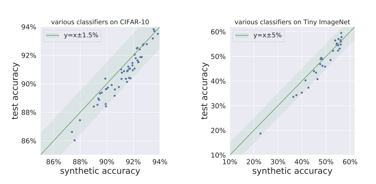
• The training speed and accuracy is only slightly worse than vanilla training: one can achieve a test accuracy of ~ 90 percent on CIFAR10 using encrypted images with a computation overhead $< 5$ percent.

• When it comes to privacy, like every other form of cryptography, its security is based upon conjectured difficulty of the underlying computational problem. (But we don’t expect breaking it to be as difficult as say breaking RSA.)

How InstaHide encryption works

Here are some details. InstaHide belongs to the class of subset-sum type encryptions (Bhattacharyya et al., 2011), and was inspired by a data augmentation technique called Mixup (Zhang et al., 2018). It views images as vectors of pixel values. With vectors you can take linear combinations. The figure below shows the result of a typical MixUp: adding 0.6 times the bird image with 0.4 times the airplane image. The image labels can also be treated as one-hot vectors, and they are mixed using the same coefficients in front of the image samples.

To encrypt the bird image, InstaHide does mixup (i.e., combination with nonnegative coefficients) with one other randomly chosen training image, and with two other images chosen randomly from a large public dataset like imagenet. The coefficients 0.6., 0.4 etc. in the figure are also chosen at random. Then it takes this composite image and for every pixel value, it randomly flips the sign. With that, we get the encrypted images and labels. All random choices made in this encryption act as a one-time key that is never re-used to encrypt other images.

InstaHide has a parameter $k$ denoting how many images are mixed; in the picture, we have $k=4$. The figure below shows this encryption mechanism.

When plugged into the standard deep learning with a private dataset of $n$ images, in each epoch of training (say $T$ epochs in total), InstaHide will re-encrypt each image in the dataset using a random one-time key. This will gives $n\times T$ encrypted images in total.

The security argument

We conjectured, based upon intuitions from computational complexity of the k-vector-subset-sum problem (citations), that extracting information about the images could time $N^{k-2}$. Here $N$, the size of the public dataset, can be tens or hundreds of millions, so it might be infeasible for real-life attackers.

We also released a challenge dataset with $k=6, n=100, T=50$ to enable further investigation of InstaHide’s security.

Carlini et al.’s recent attack on InstaHide

Recently, Carlini et al. have shared with us a manuscript with a two-step reconstruction attack (Carlini et al., 2020) against InstaHide.

TL;DR: They used 11 hours on Google’s best GPUs to get partial recovery of our 100 challenge encryptions and 120 CPU hours to break the encryption completely. Furthermore, the latter was possible entirely because we used an insecure random number generator, and they used exhaustive search over random seeds.

Now the details.

The attack takes $n\times T$ InstaHide-encrypted images as the input, ($n$ is the size of the private dataset, $T$ is the number of training epochs), and returns a reconstruction of the private dataset. It goes as follows.

• Map $n \times T$ encryptions into $n$ private images, by clustering encryptions of a same private image as a group. This is achieved by firstly building a graph representing pairwise similarity between encrypted images, and then assign each encryption a private image. In their implementation, they train a neural network to annotate pairwise similarity between encryptions.

• Then, given the encrypted images and the mapping, they solve a nonlinear optimization problem via gradient desent to recover an approximation of the original private dataset.

Using Google’s powerful GPU, it took them 10 hours to train the neural network for similarity annotation, and about another hour to get an approximation of our challenge set of $100$ images with $k=6, n=100, T=50$. This gave them vaguely correct images, with significant unclear areas and color shift.

They also proposed a different strategy which abuses the vulnerability of NumPy and PyTorch’s random number generator (Aargh; we didn’t use a secure random number generator.) They did brute force search of $2^{32}$ possible initial random seeds, which allows them to reproduce the randomness during encryption, and thus perform a pixel-perfect reconstruction. As they reported, this attack takes 120 CPU hours (they parallelize across 100 cores to obtain the solution in a little over an hour). We will have this implementation flaw fixed in an updated version.

Thoughts on this attack

Though the attack is clever and impressive, we feel that the long-term take-away is still unclear for several reasons.

Variants of InstaHide seem to evade the attack.

The challenge set contained 50 encryptions each of 100 images. This corresponds to using encrypted images for 50 epochs. But as done in existing settings that use DP, one can pretrain the deep model using non-private images and then fine-tune it with fewer epochs of the private images. Using a similar pipeline DPSGD (Abadi et al., 2016), by pretraining a ResNet-18 on CIFAR100 (the public dataset) and finetuning for $10$ epochs on CIFAR10 (the private dataset) gives accuracy of 83 percent, still far better than any provable guarantees using DP on this dataset. Carlini et al.\ team conceded that their attack probably would not work in this setting.

Similarly using InstaHide purely at inference time (i.e., using ML, instead of training ML) still should be completely secure since only one encryption of the image is released. The new attack can’t work here at all.

InstaHide was never intended to be a mission-critical encryption like RSA (which by the way also has no provable guarantees).

InstaHide is designed to give users and the internet of things a light-weight encryption method that allows them to use machine learning without giving eavesdroppers or servers access to their raw data. There is no other cost-effective alternative to InstaHide for this application. If it takes Google’s powerful computers a few hours to break our challenge set of 100 images, this is not yet a cost-effective attack in the intended settings.

More important, the challenge dataset corresponded to an ambitious form of security, where the encrypted images themselves are released to the world. The more typical application is a Federated Learning (Konečný et al., 2016) scenario: the adversary observes shared gradients that are computed using encrypted images (he also has access to the trained model). The attacks in this paper do not currently apply to that scenario. This is also the idea in TextHide, an adaptation of InstaHide to text data.

Takeways

Users need lightweight encryptions that can be applied in real time to large amounts of data, and yet allow them to take benefit of Machine Learning on the cloud. Methods to do so could completely change the privacy/utility tradeoffs implicitly assumed in today’s tech world.

InstaHide is the only such tool right now, and we now know that it provides moderate security that may be enough for many applications.

This post is based on my recent paper with Noam Razin (to appear at NeurIPS 2020), studying the question of whether norms can explain implicit regularization in deep learning. TL;DR: we argue they cannot.

Implicit regularization = norm minimization?

Understanding the implicit regularization induced by gradient-based optimization is possibly the biggest challenge facing theoretical deep learning these days. In classical machine learning we typically regularize via norms, so it seems only natural to hope that in deep learning something similar is happening under the hood, i.e. the implicit regularization strives to find minimal norm solutions. This is actually the case in the simple setting of overparameterized linear regression $-$ there, by a folklore analysis (cf. Zhang et al. 2017), gradient descent (and any other reasonable gradient-based optimizer) initialized at zero is known to converge to the minimal Euclidean norm solution. A spur of recent works (see our paper for a thorough review) has shown that for various other models an analogous result holds, i.e. gradient descent (when initialized appropriately) converges to solutions that minimize a certain (model-dependent) norm. On the other hand, as discussed last year in posts by Sanjeev as well as Wei and myself, mounting theoretical and empirical evidence suggest that it may not be possible to generally describe implicit regularization in deep learning as minimization of norms. Which is it then?

A standard test-bed: matrix factorization

A standard test-bed for theoretically studying implicit regularization in deep learning is matrix factorization $-$ matrix completion via linear neural networks. Wei and I already presented this model in our previous post, but for self-containedness I will do so again here.

In matrix completion, we are given entries $\{ M_{i, j} : (i, j) \in \Omega \}$ of an unknown matrix $M$, and our job is to recover the remaining entries. This can be seen as a supervised learning (regression) problem, where the training examples are the observed entries of $M$, the model is a matrix $W$ trained with the loss: [ \qquad \ell(W) = \sum\nolimits_{(i, j) \in \Omega} (W_{i, j} - M_{i, j})^2 ~, \qquad\qquad \color{purple}{\text{(1)}} ] and generalization corresponds to how similar $W$ is to $M$ in the unobserved locations. In order for the problem to be well-posed, we have to assume something about $M$ (otherwise the unobserved locations can hold any values, and guaranteeing generalization is impossible). The standard assumption (which has many practical applications) is that $M$ has low rank, meaning the goal is to find, among all global minima of the loss $\ell(W)$, one with minimal rank. The classic algorithm for achieving this is nuclear norm minimization $-$ a convex program which, given enough observed entries and under certain technical assumptions (“incoherence”), recovers $M$ exactly (cf. Candes and Recht).

Matrix factorization represents an alternative, deep learning approach to matrix completion. The idea is to use a linear neural network (fully-connected neural network with linear activation), and optimize the resulting objective via gradient descent (GD). More specifically, rather than working with the loss $\ell(W)$ directly, we choose a depth $L \in \mathbb{N}$, and run GD on the overparameterized objective: [ \phi ( W_1 , W_2 , \ldots , W_L ) := \ell ( W_L W_{L - 1} \cdots W_1) ~. ~~\qquad~ \color{purple}{\text{(2)}} ] Our solution to the matrix completion problem is then: [ \qquad\qquad W_{L : 1} := W_L W_{L - 1} \cdots W_1 ~, \qquad\qquad\qquad \color{purple}{\text{(3)}} ] which we refer to as the product matrix. While (for $L \geq 2$) it is possible to constrain the rank of $W_{L : 1}$ by limiting dimensions of the parameter matrices $\{ W_j \}_j$, from an implicit regularization standpoint, the case of interest is where rank is unconstrained (i.e. dimensions of $\{ W_j \}_j$ are large enough for $W_{L : 1}$ to take on any value). In this case there is no explicit regularization, and the kind of solution GD will converge to is determined implicitly by the parameterization. The degenerate case $L = 1$ is obviously uninteresting (nothing is learned in the unobserved locations), but what happens when depth is added ($L \geq 2$)?

In their NeurIPS 2017 paper, Gunasekar et al. showed empirically that with depth $L = 2$, if GD is run with small learning rate starting from near-zero initialization, then the implicit regularization in matrix factorization tends to produce low-rank solutions (yielding good generalization under the standard assumption of $M$ having low rank). They conjectured that behind the scenes, what takes place is the classic nuclear norm minimization algorithm:

Conjecture 1 (Gunasekar et al. 2017; informally stated): GD (with small learning rate and near-zero initialization) over a depth $L = 2$ matrix factorization finds solution with minimum nuclear norm.

Moreover, they were able to prove the conjecture in a certain restricted setting, and others (e.g. Li et al. 2018) later derived proofs for additional specific cases.

Two years after Conjecture 1 was made, in a NeurIPS 2019 paper with Sanjeev, Wei and Yuping Luo, we presented empirical and theoretical evidence (see previous blog post for details) which led us to hypothesize the opposite, namely, that for any depth $L \geq 2$, the implicit regularization in matrix factorization can not be described as minimization of a norm:

Conjecture 2 (Arora et al. 2019; informally stated): Given a depth $L \geq 2$ matrix factorization, for any norm $\|{\cdot}\|$, there exist matrix completion tasks on which GD (with small learning rate and near-zero initialization) finds solution that does not minimize $\|{\cdot}\|$.

Due to technical subtleties in their formal statements, Conjectures 1 and 2 do not necessarily contradict. However, they represent opposite views on the question of whether or not norms can explain implicit regularization in matrix factorization. The goal of my recent work with Noam was to resolve this open question.

Implicit regularization can drive all norms to infinity

The main result in our paper is a proof that there exist simple matrix completion settings where the implicit regularization in matrix factorization drives all norms towards infinity. By this we affirm Conjecture 2, and in fact go beyond it in the following sense: (i) not only is each norm disqualified by some setting, but there are actually settings that jointly disqualify all norms; and (ii) not only are norms not necessarily minimized, but they can grow towards infinity.

The idea behind our analysis is remarkably simple. We prove the following:

Theorem (informally stated): During GD over matrix factorization (i.e. over $\phi ( W_1 , W_2 , \ldots , W_L)$ defined by Equations $\color{purple}{\text(1)}$ and $\color{purple}{\text(2)}$), if learning rate is sufficiently small and initialization sufficiently close to the origin, then the determinant of the product matrix $W_{1: L}$ (Equation $\color{purple}{\text(3)}$) doesn’t change sign.

A corollary is that if $\det ( W_{L : 1} )$ is positive at initialization (an event whose probability is $0.5$ under any reasonable initialization scheme), then it stays that way throughout. This seemingly benign observation has far-reaching implications. As a simple example, consider the following matrix completion problem ($*$ here stands for unobserved entry): [ \qquad\qquad \begin{pmatrix} * & 1 \newline 1 & 0 \end{pmatrix} ~. \qquad\qquad \color{purple}{\text{(4)}} ] Every solution to this problem, i.e. every matrix that agrees with its observations, must have determinant $-1$. It is therefore only logical to expect that when solving the problem using matrix factorization, the determinant of the product matrix $W_{L : 1}$ will converge to $-1$. On the other hand, we know that (with probability $0.5$ over initialization) $\det ( W_{L : 1} )$ is always positive, so what is going on? This conundrum can only mean one thing $-$ as $W_{L : 1}$ fits the observations, its value in the unobserved location (i.e. $(W_{L : 1})_{11}$) diverges to infinity, which implies that all norms grow to infinity!

The above idea goes way beyond the simple example given in Equation $\color{purple}{\text(4)}$. We use it to prove that in a wide array of matrix completion settings, the implicit regularization in matrix factorization leads norms to increase. We also demonstrate it empirically, showing that in such settings unobserved entries grow during optimization. Here’s the result of an experiment with the setting of Equation $\color{purple}{\text(4)}$:

Figure 1: Solving matrix completion problem defined by Equation $\color{purple}{\text(4)}$ using matrix factorization leads absolute value of unobserved entry to increase (which in turn means norms increase) as loss decreases.

What is happening then?

If the implicit regularization in matrix factorization is not minimizing a norm, what is it doing? While a complete theoretical characterization is still lacking, there are signs that a potentially useful interpretation is minimization of rank. In our aforementioned NeurIPS 2019 paper, we derived a dynamical characterization (and showed supporting experiments) suggesting that matrix factorization is implicitly conducting some kind of greedy low-rank search (see previous blog post for details). This phenomenon actually facilitated a new autoencoding architecture suggested in a recent empirical paper (to appear at NeurIPS 2020) by Yann LeCun and his team at Facebook AI. Going back to the example in Equation $\color{purple}{\text(4)}$, notice that in this matrix completion problem all solutions have rank $2$, but it is possible to essentially minimize rank to $1$ by taking (absolute value of) unobserved entry to infinity. As we’ve seen, this is exactly what the implicit regularization in matrix factorization does!

Intrigued by the rank minimization viewpoint, Noam and I empirically explored an extension of matrix factorization to tensor factorization. Tensors can be thought of as high dimensional arrays, and they admit natural factorizations similarly to matrices (two dimensional arrays). We found that on the task of tensor completion (defined analogously to matrix completion $-$ see Equation $\color{purple}{\text(1)}$ and surrounding text), GD on a tensor factorization tends to produce solutions with low rank, where rank is defined in the context of tensors (for a formal definition, and a general intro to tensors and their factorizations, see this excellent survey by Kolda and Bader). That is, just like in matrix factorization, the implicit regularization in tensor factorization also strives to minimize rank! Here’s a representative result from one of our experiments:

Figure 2: In analogy with matrix factorization, the implicit regularization of tensor factorization (high dimensional extension) strives to find a low (tensor) rank solution. Plots show reconstruction error and (tensor) rank of final solution on multiple tensor completion problems differing in the number of observations. GD over tensor factorization is compared against "linear" method $-$ GD over direct parameterization of tensor initialized at zero (this is equivalent to fitting observations while placing zeros in unobserved locations).

So what can tensor factorizations tell us about deep learning? It turns out that, similarly to how matrix factorizations correspond to prediction of matrix entries via linear neural networks, tensor factorizations can be seen as prediction of tensor entries with a certain type of non-linear neural networks, named convolutional arithmetic circuits (in my PhD I worked a lot on analyzing the expressive power of these models, as well as showing that they work well in practice $-$ see this survey for a soft overview).

Figure 3: The equivalence between matrix factorizations and linear neural networks extends to an equivalence between tensor factorizations and a certain type of non-linear neural networks named convolutional arithmetic circuits.

Analogously to how the input-output mapping of a linear neural network can be thought of as a matrix, that of a convolutional arithmetic circuit is naturally represented by a tensor. The experiment reported in Figure 2 (and similar ones presented in our paper) thus provides a second example of a neural network architecture whose implicit regularization strives to lower a notion of rank for its input-output mapping. This leads us to believe that implicit rank minimization may be a general phenomenon, and developing notions of rank for input-output mappings of contemporary models may be key to explaining generalization in deep learning.

Nadav Cohen

In our previous blog post, we introduced the challenges of sampling distributions beyond log-concavity. We first introduced the problem of sampling from a distibution $p(x) \propto e^{-f(x)}$ given value or gradient oracle access to $f$, as an analogous problem to black-box optimization with oracle access. We introduced the natural algorithm for sampling in this setup: Langevin Monte Carlo, a Markov Chain reminiscent of noisy gradient descent,

Finally, we laid out the challenges when $f$ is not convex; in particular, LMC can suffer from slow mixing.

In this and the coming post, we describe two of our recent works tackling this problem. We identify two kinds of structure beyond log-concavity under which we can design provably efficient algorithms: multi-modality and manifold structure in the level sets. These structures commonly occur in practice, especially in problems involving statistical inference and posterior sampling in generative models.

In this post, we will focus on multimodality, covered by the paper Simulated tempering Langevin Monte Carlo by Rong Ge, Holden Lee, and Andrej Risteski.

Sampling multimodal distributions with simulated tempering

The classical scenario in which Langevin takes exponentially long to mix is when $p$ is a mixture of two well-separated gaussians. In broadest generality, this was considered by Bovier et al. 2004 who used tools from metastable processes to show that transitioning from one peak to another can take exponential time. Roughly speaking, they show the transition time is proportional to the “energy barrier” a particle has to cross. If the gaussians have unit variance and means at distance $2r$, then the probability density at a point midway in between is $\propto e^{-r^2/2}$, and this energy barrier is $\propto e^{r^2/2}$. Thus, the mixing time is exponential. Qualitatively, the intuition for this phenomenon is simple to describe: if started at point A, the drift (i.e. gradient) term will push the walk towards A, so long as it’s close to the basin around A; hence, to transition from A to B (through C) the Gaussian noise must persistenly counteract the gradient term.

Hence Langevin on its own will not work even in very simple multimodal settings.

In our paper, we show that combining Langevin Monte Carlo with a temperature-based heuristic called simulated tempering can significantly speed up mixing for multimodal distributions, where the number of modes is not too large, and the modes “look similar.”

More precisely, we show:

Theorem (Ge, Lee, Risteski ‘18, informal): If $p(x)$ is a mixture of $k$ shifts of a strongly log-concave distribution in $d$ dimensions (e.g. Gaussian), an algorithm based on simulated tempering and Langevin Monte Carlo that runs in time poly($d,k, 1/\varepsilon$) produces samples from a distribution $\varepsilon$-close to $p$ in total variation distance.

The main idea is to create a meta-Markov chain (the simulated tempering chain) which has two types of moves: change the current “temperature” of the sample, or move “within” a temperature. The main intuition behind this is that at higher temperatures, the distribution is flatter, so the chain explores the landscape faster (see the figure below).

More formally, the distribution at inverse temperature $\beta$ is given by $p_\beta(x) \propto e^{-\beta f(x)}$. The Langevin chain which corresponds to $\beta$ is given by

As in the figure above, a high temperature (low $\beta<1$) flattens out the distribution and causes the chain to mix faster (top distribution in figure). However, we can’t merely run Langevin at a higher temperature, because the stationary distribution of the high-temperature chain is wrong: it’s $p_\beta(x)$. The idea behind simulated tempering is to run Langevin chains at different temperatures, sometimes swapping to another temperature to help lower-temperature chains explore. To maintain the right stationary distributions at each temperature, we use a Metropolis-Hastings filtering step.

More formally, choosing a suitable sequence $0< \beta_1< \cdots <\beta_L=1$, we define the simulated tempering chain as follows.

• The state space is a pair of a temperature and location in space $(i, x), i \in [L], x \in \mathbb{R}^d$.
  
• The transitions are defined as follows.
  • If the current point is $(i,x)$, then evolve $x$ according to Langevin diffusion with inverse temperature $\beta_i$.
  • Propose swaps with some rate $\lambda >0$. Proposing a swap means attempting to move to a neighboring chain, i.e. change $i$ to $i’=i\pm 1$. With probability $\min{p_{i’}(x)/p_i(x), 1}$, the transition is accepted. Otherwise, stay at the same point. This is a Metropolis-Hastings step; its purpose is to preserve the stationary distribution.

Finally, it’s not too hard to see that at the stationary distribution, the samples at the $L$th level ($\beta_L=1$) are the desired samples.

Proof idea: decomposition theorem

The main strategy is inspired by Madras and Randall’s Markov chain decomposition theorem, which gives a criterion for a Markov chain to mix rapidly: partition the state space into sets, and show that

1. The Markov chain mixes rapidly when restricted to each set of the partition.
2. The projected Markov Chain, which we define momentarily, mixes rapidly. If there are $m$ sets, the projected chain $\overline M$ is defined on the state space ${1,\ldots, m}$, and transition probabilities are given by average probability flows between the corresponding sets.

To implement this strategy, we first have to specify the partition. In fact, we roughly show that there is a partition of $[L] \times \mathbb{R}^d$ in which:

1. The simulated tempering Langevin chain mixes fast within each of the sets.
2. The “volume” of the sets (under the stationary distribution of the tempering chain) is not too small.

In applying the Madras-Randall framework with this partition, it’s clear that point (1) above satisfies requirement (1) for the framework; point (2) ensures that the projected Markov chain has no “bottlenecks” and hence that it mixes rapidly (requirement (2)). More precisely, we can show rapid mixing either through the method of canonical paths or Cheeger’s inequality. To do this, we exhibit a “good-probability” path between any two sets in the partition, going through the highest temperature.

The intuition for why this path works is illustrated in the figure below: when transitioning from the set corresponding to the left mode at level $L$ to the right mode at level $L$, each of the steps up/down the temperatures are accepted with good probability if the neighboring temperatures are not too different; at the highest temperature, the chain mixes fast by point (1), and since each of the sets are not too small by point (2), there is a reasonable probability to end at the right mode at the highest temperature.

Intuitively, the partition should track the “modes” of the distribution, but a technical hurdle in implementing this plan is in defining the partition when the modes overlap. One can either do this spectrally (i.e. showing that the Langevin chain has a spectral gap, and use theorems about spectral graph partitioning, as we did in the first version of the paper), or use a functional “soft decomposition theorem” which is a more flexible version of the classical decomposition theorem, which we use in a later version of the paper.

In the first post of this series, we introduced the challenges of sampling distributions beyond log-concavity. In Part 2 we tackled sampling from multimodal distributions: a typical obstacle occuring in problems involving statistical inference and posterior sampling in generative models. In this (final) post of the series, we consider sampling in the presence of manifold structure in the level sets of the distribution– which also frequently manifests in the same settings. It will cover the paper Fast convergence for Langevin diffusion with matrix manifold structure by Ankur Moitra and Andrej Risteski .

Sampling with matrix manifold structure

The structure on the distribution we consider in this post is manifolds of equiprobable points: this is natural, for instance, in the presence of invariances in data (e.g. rotations of images). It can also appear in neural-network based probabilistic models due to natural invariances they encode (e.g., scaling invariances in ReLU-based networks).

At the level of techniques, the starting point for our results is a close connection between the geometry, more precisely Ricci curvature of a manifold, and the mixing time of Brownian motion on a manifold. The following theorem holds:

Theorem (Bakry and Émery ‘85, informal): If the manifold $M$ has positive Ricci curvature, Brownian motion on the manifold mixes rapidly in $\chi^2$ divergence.

We will explain the notions from differential geometry shortly, but first we sketch our results, and how they use this machinery. We present two results: the first is a “meta”-theorem that provides a generic decomposition framework, and the second is an instantiation of this framework for a natural family of problems that exhibit manifold structure: posteriors for matrix factorization, sensing, and completion.

A general manifold decomposition framework

Our first result is a general decomposition framework for analyzing mixing time of Langevin in the presence of manifolds of equiprobable points.

To motivate the result, note that if we consider the distribution $p_{\beta}(x) \propto e^{-\beta f(x)}$, for large (but finite) $\beta$, the Langevin chain corresponding to that distribution, started close to a manifold of local minima, will tend to stay close to (but not on!) it for a long time. See the figure below for an illustration. This, we will state a “robust” version of the above manifold result, for a chain that’s allowed to go off the manifold.

We show the following statement. (Recall that a bounded Poincaré constant corresponds to rapid mixing for Langevin. See the first post for a refresher.)

Theorem 1 (Moitra and Risteski ‘20, informal): Suppose the Langevin chain corresponding to $p(x) \propto e^{-f(x)}$ is initialized close to a manifold $M$ satisfying the following two properties:

(1) It stays in some neighborhood $D$ of the manifold $M$ with large probability for a long time.

(2) $D$ can be partitioned into manifolds $M^{\Delta}$ satisfying:

(2.1) The conditional distribution of $p$ restricted to $M^{\Delta}$ has a upper bounded Poincare constant.

(2.2) The marginal distribution over $\Delta$ has a upper bounded Poincare constant.

(2.3) The conditional probability distribution over $M^{\Delta}$ does not “change too quickly” as $\Delta$ changes.

Then Langevin mixes quickly to a distribution close to the conditional distribution of $p$ restricted to $D$.

While the above theorem is a bit of a mouthful (even very informally stated) and requires a choice of partitioning of $D$ to be “instantiated”, it’s quite natural to think of it as an analogue of local convergence results for gradient descent in optimization. Namely, it gives geometric conditions under which Langevin started near a manifold mixes to the “local” stationary distribution (i.e. the conditional distribution $p$ restricted to $D$).

The proof of the theorem uses similar decomposition ideas as result on sampling multimodal distributions from the previous post, albeit is complicated by measure theoretic arguments. Namely, the manifolds $M^{\Delta}$ have technically zero measure under the distribution $p$, so care must be taken with how the “projected” and “restricted” chain are defined—the key tool for this is the so-called co-area formula.

The challenge in using the above framework is instantiating the decomposition: namely, the choice of the partition of $D$ into manifolds $M^{\Delta}$. In the next section, we show how this can be done for posteriors in problems like matrix factorization/sensing/completion.

Matrix factorization (and relatives)

To instantiate the above framework in a natural setting, we consider distributions exhibiting invariance under orthogonal transformations. Namely, we consider distributions of the type

where $b \in \mathbb{R}^{m}$ is a fixed vector and $\mathcal{A}$ is an operator that returns a $m$-dimensional vector given a $d \times d$ matrix. For this distribution, we have $p(X) = p(XO)$ for any orthogonal matrix $O$, since $XX^T = XO (XO)^T$ . Depending on the choice of $\mathcal{A}$, we can easily recover some familiar functions inside the exponential: e.g. the $l_2$ losses for (low-rank) matrix factorization, matrix sensing and matrix completion. These losses received a lot of attention as simple examples of objectives that are non-convex but can still be optimized using gradient descent. (See e.g. Ge et al. ‘17.)

These distributions also have a very natural statistical motivation. Namely, consider the distribution over $m$-dimensional vectors, such that

Then, the distribution $p(X) \propto e^{-\beta | \mathcal{A}(XX^T) - b |^2_2 }$ can be viewed as the posterior distribution over $X$ with a uniform prior. Thus, sampling from these distributions can be seen as the distributional analogue of problems like matrix factorization/sensing/completion, the difference being that we are not merely trying to find the most likely matrix $X$, but also trying to sample from the posterior.

We will consider the case when $\beta$ is sufficiently large (in particular, $\beta = \Omega(\mbox{poly}(d))$: in this case, the distribution $p$ will concentrate over two (separated) manifolds: $E_1 = \{X_0 R: R \mbox{ is orthogonal with det 1}\}$ and $E_2 = \{X_0 R: R \mbox{ is orthogonal with det }-1\}$, where $X_0$ is any fixed minimizer of $| \mathcal{A}(XX^T) - b |^2_2$. Hence, when started near one of these manifolds, we expect Langevin to stay close to it for a long time (see figure below).

We show:

Theorem 2 (Moitra and Risteski ‘20, informal): Let $\mathcal{A}$ correspond to matrix factorization, sensing or completion under standard parameter assumptions for these problems. Let $\beta = \Omega(\mbox{poly}(d))$. If initialized close to one of $E_i, i \in \{1, 2\}$, after a polynomial number of steps the discretized Langevin dynamics will converge to a distribution that is close in total variation distance to p(X) when restricted to a neighborhood of $E_i$.

We remark that the closeness condition for the first step is easy to ensure using existing results on gradient-descent based optimization for these objectives. It’s also easy to use the above result to sample approximately from the distribution $p$ itself, rather than only the “local” distributions $p^i$ – this is due to the fact that the distribution $p$ looks like the “disjoint union” of the distributions $p^1$ and $p^2$.

Before we describe the main elements of the proof, we review some concepts from differential geometry.

(Extremely) brief intro to differential geometry

We won’t do a full primer on differential geometry in this blog post, but we will briefly informally describe some of the relevant concepts. See Section 5 of our paper for an intro to differential geometry (written with a computer science reader in mind, so more easy-going than a differential geometry textbook).

Recall, the tangent space at $x$, denoted by $T_x M$, is the set of all derivatives $v$ of a curve passing through $x$. The Ricci curvature at a point $x$, in direction $v \in T_x M$, denoted $\mbox{Ric}_x(v)$, captures the second-order term in the rate of change of volumes of sets in a small neighborhood around $x$, as the points in the set are moved along the geodesic (i.e. shortest path curve) in direction $v$ (or more precisely, each point $y$ in the set is moved along the geodesic in the direction of the parallel transport of $v$ at $y$; see the right part of the figure below from (Ollivier 2010)). A Ricci curvature of $0$ preserves volumes (think: a plane), a Ricci curvature $>0$ shrinks volume (think: a sphere), and a Ricci curvature $<0$ expands volume (think: a hyperbola).

The connections between curvature and mixing time of diffiusions is rather deep and we won’t attempt to convey it fully in a blog post - the definitive reference is Analysis and Geometry of Markov Diffusion Operators by Bakry, Gentil and Ledoux. The main idea is that mixing time can be bounded by how long it takes for random walks starting at different locations to “join together,” and positive curvature brings them together faster.

To make this formal, we define a coupling of two random variables $X, Y$ to be any random variable $W = (X’,Y’)$ such that the marginal distribution of the coordinates $X’$ and $Y’$ are the same as the distributions of $X$ and $Y$. It’s well known that the convergence time of a random walk in total variation distance can be upper bounded by the expected time until two coupled copies of the walk join. On the plane, a canonical coupling (the reflection coupling) between two Brownian motions can be constructed by reflecting the move of the second process through the perpendicular bisector between the locations of the two processes (see figure below). On a positively curved manifold (like a sphere), an analogous reflection can be defined, and the curvature only brings the two processes closer faster.

As a final tool, our proof uses a very important theorem due to Milnor about manifolds with algebraic structure:

Theorem (Milnor ‘76, informal): The Ricci curvature of a Lie group equipped with a left-invariant metric is non-negative.

In a pinch, a Lie group is a group that also is a smooth manifold, and furthermore, the group operations result in a smooth transformation on the manifold - so that the “geometry” and “algebra” combine together. A metric is left-invariant for the group if acting on the left by any group element leaves the metric “unchanged”.

Implementing the decomposition framework

To apply the framework we sketched out as part of Theorem 1, we need to verify the conditions of the Theorem.

To prove Condition 1, we need to show that for large $\beta$, the random walk stays near to the manifold it’s been initialized close to. The main tools for this are Ito’s lemma, local convexity of the function $| \mathcal{A}(XX^T) - b |_2^2$ and basic results in the theory of Cox-Ingersoll-Ross processes. Namely, Ito’s lemma (which can be viewed as a “change-of-variables” formula for random variables) allows us to write down a stochastic differential equation for the evolution of the distance of $X$ from the manifold, which turns out to have a “bias” towards small values, due to the local convexity of $| \mathcal{A}(XX^T) - b |_2^2$. This can in turn be analyzed approximately as Cox-Ingersoll-Ross process - a well-studied type of non-negative stochastic process.

To prove Condition 2, we need to specify the partition of the space around the manifolds $E_i$. Describing the full partition is somewhat technical, but importantly, the manifolds $M^{\Delta}$ have the form $M^{\Delta} = \{\Delta U: U \mbox{ is an orthogonal matrix with det 1}\}$ for some matrix $\Delta \in \mathbb{R}^{n \times k}$.

The proof that $M^{\Delta}$ has a good Poincare constant (i.e. Condition 2.1) relies on two ideas: first, $M^{\Delta}$ is a Lie group with group operation $\circ$ defined such that $(\Delta U) \circ (\Delta V) := \Delta (UV)$, along with a corresponding left-invariant metric - thus, by Milnor’s theorem, it has a non-negative Ricci curvature; second, we can relate the Ricci curvatures with the Euclidean metric to the curvature with the left-invariant metric. The proof that the marginal distribution over $\Delta$ has a good Poincaré constant involves showing that this distribution is approximately log-concave. Finally, the “change-of-conditional-probability” condition (Condition 2.3) can be proved by explicit calculation.

Closing remarks

In this series of posts, we surveyed two recent approaches to analyzing Langevin-like sampling algorithms beyond log-concavity - the most natural analogue to non-convexity in the world of sampling/inference. The structures we considered, multi-modality and invariant manifolds, are common in practice in modern machine learning.

Unlike non-convex optimization, provable guarantees for sampling beyond log-concavity is still under-studied and we hope our work will inspire and excite further efforts. For instance, how do we handle modes of different “shape”? Can we handle an exponential number of modes, if they have further structure (e.g., posteriors in concrete latent-variable models like Bayesian networks)? Can we handle more complex manifold structure (e.g. the matrix distributions we considered for any $\beta$)?

The empirical success of deep learning has posed significant challenges to machine learning theory: Why can we efficiently train neural networks with gradient descent despite its highly non-convex optimization landscape? Why do over-parametrized networks generalize well? The recently proposed Neural Tangent Kernel (NTK) theory offers a powerful framework for understanding these, but yet still comes with its limitations.

In this blog post, we explore how to analyze wide neural networks beyond the NTK theory, based on our recent Beyond Linearization paper and follow-up paper on understanding hierarchical learning. (This blog post is also cross-posted at the Salesforce Research blog.)

Neural Tangent Kernels

The Neural Tangent Kernel (NTK) is a recently proposed theoretical framework for establishing provable convergence and generalization guarantees for wide (over-parametrized) neural networks (Jacot et al. 2018). Roughly speaking, the NTK theory shows that

• A sufficiently wide neural network trains like a linearized model governed by the derivative of the network with respect to its parameters.
• At the infinite-width limit, this linearized model becomes a kernel predictor with the Neural Tangent Kernel (the NTK).

Consequently, a wide neural network trained with small learning rate converges to 0 training loss and generalize as well as the infinite-width kernel predictor. For a detailed introduction to the NTK, please refer to the earlier blog post by Wei and Simon.

Does NTK fully explain the success of neural networks?

Although the NTK yields powerful theoretical results, it turns out that real-world deep learning do not operate in the NTK regime:

• Empirically, infinite-width NTK kernel predictors perform slightly worse (though competitive) than fully trained neural networks on benchmark tasks such as CIFAR-10 (Arora et al. 2019b). For finite width networks in practice, this gap is even more profound, as we see in Figure 1: The linearized network is a rather poor approximation of the fully trained network at practical optimization setups such as large initial learning rate (Bai et al. 2020).
• Theoretically, the NTK has poor sample complexity for learning certain simple functions. Though the NTK is a universal kernel that can interpolate any finite, non-degenerate training dataset (Du et al. 2018, 2019), the test error of this kernel predictor scales with the RKHS norm of the ground truth function. For certain non-smooth but simple functions such as a single ReLU, this norm can be exponentially large in the feature dimension (Yehudai & Shamir 2019). Consequently, NTK analyses yield poor sample complexity upper bounds for learning such functions, whereas empirically neural nets only require a mild sample size (Livni et al. 2014).

Figure 1. Linearized model does not closely approximate the training trajectory of neural networks with practical optimization setups, whereas higher order Taylor models offer a substantially better approximation.

These gaps urge us to ask the following

Question: How can we theoretically study neural networks beyond the NTK regime? Can we prove that neural networks outperform the NTK on certain learning tasks?

The key technical question here is to mathematically understand neural networks operating outside of the NTK regime.

Higher-order Taylor expansion

Our main tool for going beyond the NTK is the Taylor expansion. Consider a two-layer neural network with $m$ neurons, where we only train the “bottom” nonlinear layer $W$:

(Here, $W_0+W$ is an $m\times d$ weight matrix, where $W_0$ denotes the random initialization and $W$ denotes the trainable “movement” matrix initialized at zero). For small enough $W$, we can perform a Taylor expansion of the network around $W_0$ and get

Let us denote the $k$-th order term as $ f^{(k)}_{W_0, W}$, and rewrite this as

Above, term $f^{(k)}$ is a $k$-th order polynomial of the trainable parameter $W$. For the moment assume that $f^{(0)}(x)=0$ (this can be achieved via techniques such as the symmetric initialization).

The key insight of the NTK theory can be described as the following linearized approximation property

For small enough $W$, the neural network $f_{W_0,W}$ is closely approximated by the linear model $f^{(1)}$.

Towards moving beyond the linearized approximation, in our Beyond Linearization paper, we start by asking

Why just $f^{(1)}$? Can we also utilize the higher-order term in the Taylor series such as $f^{(2)}$?

At first sight, this seems rather unlikely, as in Taylor expansions we always expect the linear term $f^{(1)}$ to dominate the whole expansion and have a larger magnitude than $f^{(2)}$ (and subsequent terms).

“Killing” the NTK term by randomized coupling

We bring forward the idea of randomization, which helps us escape the “domination” of $f^{(1)}$ and couple neural networks with their quadratic Taylor expansion term $f^{(2)}$. This idea appeared first in Allen-Zhu et al. (2018) for analyzing three-layer networks, and as we will show also applies to two-layer networks in a perhaps more intuitive fashion.

Let us now assign each weight movement $w_r$ with a random sign $s_r\in\{\pm 1\}$, and consider the randomized weights $\{s_rw_r\}$. The random signs satisfy the following basic properties:

Therefore, let $SW\in\mathbb{R}^{m\times d}$ denote the randomized weight matrix, we can compare the first and second order terms in the Taylor expansion at $SW$:

whereas

Observe that the sign randomization keeps the quadratic term $f^{(2)}$ unchanged, but “kills” the linear term $f^{(1)}$ in expectation!

If we train such a randomized network with freshly sampled signs $S$ at each iteration, the linear term $f^{(1)}$ will keep oscillating around zero and does not have any power in fitting the data, whereas the quadratic term is not affected at all and thus becomes the leading force for fitting the data. (The keen reader may notice that this randomization is similar to Dropout, with the key difference being that we randomize the weight movement matrix, whereas vanilla Dropout randomizes the weight matrix itself.)

Figure 2. The NTK regime operates in the "NTK ball" where the network is approximately equal to the linear term. The quadratic regime operates in a larger ball where the network is approximately equal to the sum of first two terms, but the linear term dominates and can blow up at large width. Our randomized coupling technique resolves this by introducing the random sign matrix that in expectation "kills" the linear term but always preserves the quadratic term.

Our first result shows that networks with sign randomization can still be efficiently optimized, despite its now non-convex optimization landscape:

Theorem: Any escaping-saddle algorithm (e.g. noisy SGD) on the regularized loss function $E_S[L(W_0+SW)]+R(W)$, with freshly sampled sign $S=S_t$ per iteration, can find the global minimum in polynomial time.

The proof builds on the quadratic approximation $E_S[f]\approx f^{(2)}$ and recent understandings on neural networks with quadratic activation, e.g. Soltanolkotabi et al. (2017)& Du and Lee (2018).

Generalization and sample complexity: Case study on learning low-rank polynomials

We next study the generalization of these networks in the context of learning low-rank degree-$p$ polynomials:

We are specifically interested in the case where $r_\star$ is small (e.g. $O(1)$), so that $y$ only depends on the projection of $x$ on a few directions. This for example captures teacher networks with polynomial activation of bounded degree and analytic activation (approximately), as well as constant depth teacher networks with polynomial activations.

For the NTK, the sample complexity of learning polynomials have been studied extensively in (Arora et al. 2019a), (Ghorbani et al. 2019), and many concurrent work. Combined, they showed that the sample complexity for learning degree-$p$ polynomials is $\Theta(d^p)$, with matching lower and upper bounds:

Theorem (NTK) : Suppose $x$ is uniformly distributed on the sphere, then the NTK requires $O(d^p)$ samples in order to achieve a small test error for learning any degree-$p$ polynomial, and there is a matching lower bound of $\Omega(d^p)$ for any inner-product kernel method.

In our Beyond Linearization paper, we show that the quadratic Taylor model achieves an improved sample complexity of $\tilde{O}(d^{p-1})$ with isotropic inputs:

Theorem (Quadratic Model): For mildly isotropic input distributions, the two-layer quadratic Taylor model (or two-layer NN with sign randomization) only requires $\tilde{O}({\rm poly}(r_\star, p)d^{p-1})$ samples in order to achieve a small test error for learning a low-rank degree-$p$ polynomial.

In our follow-up paper on understanding hierarchical learning, we further design a “hierarchical learner” using a specific three-layer network, and show the following

Theorem (Three-layer hierarchical model): Under mild input distribution assumptions, a three-layer network with a fixed representation layer of width $D=d^{p/2}$ and a trainable quadratic Taylor layer can achieve a small test error using only $\tilde{O}({\rm poly}(r_\star, p)d^{p/2})$ samples.

When $r_\star,p=O(1)$, the quadratic Taylor model can improve over the NTK by a multiplicative factor of $d$, and we can further get a substantially larger improvement of $d^{p/2}$ by using the three-layer hierarchical learner. Here we briefly discuss the proof intuitions, and refer the reader to our papers for more details.

• Generalization bounds: We show that, while the NTK and quadratic Taylor model expresses functions using similar random feature constructions, their generalization depends differently on the norm of the input. In the NTK, the generalization depends on the L2 norm of the features (as well as the weights), whereas generalization of the quadratic Taylor model depends on the operator norm of the input matrix features $\frac{1}{n}\sum x_ix_i^\top$ times the nuclear norm of $\sum w_rw_r^\top$. It turns out that this decomposition can match the one given by the NTK (it is never worse), and in addition be better by a factor of $O(\sqrt{d})$ if the input distribution is mildly isotropic so that $\|\frac{1}{n}\sum x_ix_i^\top\|_{\rm op} \le 1/\sqrt{d} \cdot \max \|x_i\|_2^2$, leading to the $O(d)$ improvement in the sample complexity.

• Hierarchical learning: The key intuition behind the hierarchical learner is that we can utilize the $O(d)$ sample complexity gain to its fullest, by applying quadratic Taylor model to not the input $x$, but a feature representation $h(x)\in \mathbb{R}^D$ where $D\gg d$. This yields a gain as long as $h$ is rich enough to express $f_\star$ and also isotropic enough to let the operator norm $\|\frac{1}{n}\sum h(x_i)h(x_i)^\top\|_{\rm op}$ be nice. In particular, for learning degree-$p$ polynomials, the best we can do is to choose $D=d^{p/2}$, leading to a sample complexity saving of $\tilde{O}(D)=\tilde{O}(d^{p/2})$.

Concluding thoughts

In this post, we explored higher-order Taylor expansions (in particular the quadratic expansion) as an approach to deep learning theory beyond the NTK regime. The Taylorization approach has several advantages:

• Non-convex but benign optimization landscape;
• Provable generalization benefits over NTKs;
• Ability of modeling hierarchical learning;
• Convenient API for expeirmentation (cf. the Neural Tangents package and the Taylorized training paper).

We believe these advantages make the Taylor expansion a powerful tool for deep learning theory, and our results are just a beginning. We also remark that there are other theoretical frameworks such as the Neural Tangent Hierarchy or the Mean-Field Theory that go beyond the NTK with their own advantages in various angles, but without computational efficiency guarantees. See the slides for more on going beyond NTK. Making progress on any of these directions (or coming up with new ones) would be an exciting direction for future work.

Can you trust a model whose designer had access to the test/holdout set? This implicit question in Dwork et al 2015 launched a new field, adaptive data analysis. The question referred to the fact that in many scientific settings as well as modern machine learning (with its standardized datasets like CIFAR, ImageNet etc.) the model designer has full access to the holdout set and is free to ignore the

(Basic Dictum of Data Science) “Thou shalt not train on the test/holdout set.”

Furthermore, even researchers who scrupulously follow the Basic Dictum may be unknowingly violating it when they take inspiration (and design choices) from published works by others who presumably published only the best of the many models they evaluated on the test set.

Dwork et al. showed that if the test set has size $N$, and the designer is allowed to see the error of the first $i-1$ models on the test set before designing the $i$’th model, then a clever designer can use so-called wacky boosting (see this blog post) to ensure the accuracy of the $t$’th model on the test set as high as $\Omega(\sqrt{t/N})$. In other words, the test set could become essentially useless once $t \gg N$, a condition that holds in ML, whereby in popular datasets (CIFAR10, CIFAR100, ImageNet etc.) $N$ is no more than $100,000$ and the total number of models being trained world-wide is well in the millions if not higher (once you include hyperparameter searches).

Meta-overfitting Error (MOE) of a model is the difference between its average error on the test data and its expected error on the full distribution. (It is closely related to false discovery rate in statistics.)

This blog post concerns our new paper, which gives meaningful upper bounds on this sort of trouble for popular deep net architectures, whereas prior ideas from adaptive data analysis gave no nontrivial estimates. We call our estimate Rip van Winkle’s Razor which combines references to Occam’s Razor and the mythical person who fell asleep for 20 years.

Adaptive Data Analysis: Brief tour

It is well-known that for a model trained without ever querying the test set, MOE scales (with high probability over choice of the test set) as $1/\sqrt{N}$ where $N$ is the size of the test set. Furthermore standard concentration bounds imply that even if we train $t$ models without ever referring to the test set (in other words, using proper data hygiene) then the maximum meta-overfitting error among the $t$ models scales whp as $O(\sqrt{\log(t)/ N})$. The trouble pinpointed by Dwork et al. can happen only if models are designed adaptively, with test error of the previous models shaping the design of the next model.

Adaptive Data Analysis has come up with many good practices for honest researchers to mitigate such issues. For instance, Dwork et al. showed that using Differential Privacy on labels while evaluating models can lower MOE. Or the Ladder mechanism helps in Kaggle-like settings where the test dataset resides on a server that can choose to answers only a selected subset of queries, which essentially takes away the MOE issue.

For several good practices matching lower bounds exist showing a way to construct cheating models with MOE matching the upper bound.

However such recommended best practices do not help with understanding the MOE in the performance numbers of a new model since there is no guarantee that the inventors never tuned models using the test set, or didn’t get inspiration from existing models that may have been designed that way. Thus statistically speaking the above results still give no reason to believe that a modern deep net such as ResNet152 has low MOE.

Recht et al. 2019 summed up the MOE issue in a catchy title: Do ImageNet Classifiers Generalize to ImageNet? They tried to answer their question experimentally by creating new test sets from scratch –we discuss their results later.

MOE bounds and description length

The starting point of our work is the following classical concentration bounds:

Folklore Theorem With high probability over the choice of a test set of size $N$, the MOE of all models with description length at most $k$ bits is $O(\sqrt{k/N})$.

At first sight this doesn’t seem to help us because one cannot imagine modern deep nets having a short description. The most obvious description involves reporting values of the net parameters, which requires millions or even hundreds of millions of bits, resulting in a vacuous upper bound on MOE.

Another obvious description would be the computer program used to produce the model using the (publicly available) training and validation sets. However, these programs usually rely on imported libraries through layers of encapsulation and so the effective program size is pretty large as well.

Rip van Winkle’s Razor

Our new upper bound involves a more careful definition of Description Length: it is the smallest description that allows a referee to reproduce a model of similar performance using the (universally available) training and validation datasets.

While this phrasing may appear reminiscent of the review process for conferences and journals, there is a subtle difference with respect to what the referee can or cannot be assumed to know. (Clearly, assumptions about the referee can greatly affect description length —e.g, a referee ignorant of even basic calculus might need a very long explanation!)

Informed Referee:“Knows everything that was known to humanity (e.g., about deep learning, mathematics,optimization, statistics etc.) right up to the moment of creation of the Test set.”

Unbiased Referee: Knows nothing discovered since the Test set was created.

Thus Description Length of a model is the number of bits in the shortest description that allows an informed but unbiased referee to reproduce the claimed result.

Note that informed referees let descriptions get shorter. Unbiased require longer descriptions that rule out any statistical “contamination” due to any interaction whatsoever with the test set. For example, momentum techniques in optimization were well-studied before the creation of ImageNet test set, so informed referees can be expected to understand a line like “SGD with momentum 0.9.” But a line like “Use Batch Normalization” cannot be understood by unbiased referees since conceivably this technique (invented after 2012) might have become popular precisely because it leads to better performance on the test set of ImageNet.

By now it should be clear why the estimate is named after “Rip van Winkle”: the referee can be thought of as an infinitely well-informed researcher who went into deep sleep at the moment of creation of the test set, and has just been woken up years later to start refereeing the latest papers. Real-life journal referees who luckily did not suffer this way should try to simulate the idealized Rip van Winkle in their heads while perusing the description submitted by the researcher.

To allow as short a description as possible the researcher is allowed to compress the description of their new deep net non-destructively using any compression that would make sense to Rip van Winkle (e.g., Huffman Coding). The description of the compression method itself is not counted towards the description length – provided the same method is used for all papers submitted to Rip van Winkle. To give an example, a technique appearing in a text known to Rip van Winkle could be succinctly referred to using the book’s ISBN number and page number.

Estimating MOE of ResNet-152

As an illustration, here we provide a suitable description allowing Rip van Winkle to reproduce a mainstream ImageNet model, ResNet-152, which achieves $4.49\%$ top-5 test error.

The description consists of three types of expressions: English phrases, Math equations, and directed graphs. In the paper, we describe in detail how to encode each of them into binary strings and count their lengths. The allowed vocabulary includes primitive concepts that were known before 2012, such as CONV, MaxPool, ReLU, SGD etc., as well as a graph-theoretic notation/shorthand for describing net architecture. The newly introduced concepts including Batch-Norm, Layer, Block are defined precisely using Math, English, and other primitive concepts.

According to our estimate, the length of the above description is $1032$ bits, which translates into a upper bound on meta-overfitting error of merely $5\%$! This suggests the real top-5 error of the model on full distribution is at most $9.49\%$. In the paper we also provide a $980$-bit long description for reproducing DenseNet-264, which leads to $5.06\%$ upper bound on its meta-overfitting error.

Note that the number $5.06$ suggests higher precision than actually given by the method, since it is possible to quibble about the coding assumptions that led to it. Perhaps others might use a more classical coding mechanism and obtain an estimate of $6\%$ or $7\%$.

But the important point is that unlike existing bounds in Adaptive Data Analysis, there is no dependence on $t$, the number of models that have been tested before, and the bound is non-vacuous.

Empirical evidence about lack of meta-overfitting

Our estimates indicate that the issue of meta-overfitting on ImageNet for these mainstream models is mild. The reason is that despite the vast number of parameters and hyper-parameters in today’s deep nets, the information content of these models is not high given knowledge circa 2012.

Recently Recht et al. tried to reach an empirical upper bound on MOE for ImageNet and CIFAR-10. They created new tests sets by carefully replicating the methodology used for constructing the original ones. They found that error of famous published models of the past seven years is as much as 10-15% higher on the new test set as compared to the original. On the face of it, this seemed to confirm a case of bad meta-overfitting. But they also presented evidence that the swing in test error was due to systemic effects during test set creation. For instance, a comparable swing happens also for models that predated the creation of ImageNet (and thus were not overfitted to the ImageNet test set). A followup study of a hundred Kaggle competitions used fresh, identically distributed test sets that were available from the official competition organizers. The authors concluded that MOE does not appear to be significant in modern ML.

Conclusions

To us the disquieting takeaway from Recht et al.’s results was that estimating MOE by creating a new test set is rife with systematic bias at best, and perhaps impossible, especially in datasets concerning rare or one-time phenomena (e.g., stock prices). Thus their work still left a pressing need for effective upper bounds on meta-overfitting error. Our Rip van Winkle’s Razor is elementary, and easily deployable by the average researcher. We hope it becomes part of the standard toolbox in Adaptive Data Analysis.

In effort to understand implicit regularization in deep learning, a lot of theoretical focus is being directed at matrix factorization, which can be seen as linear neural networks. This post is based on our recent paper (to appear at ICML 2021), where we take a step towards practical deep learning, by investigating tensor factorization— a model equivalent to a certain type of non-linear neural networks. It is well known that most tensor problems are NP-hard, and accordingly, the common sentiment is that working with tensors (in both theory and practice) entails extreme difficulties. However, by adopting a dynamical systems view, we manage to avoid such difficulties, and establish an implicit regularization towards low tensor rank. Our results suggest that tensor rank may shed light on generalization in deep learning.

Challenge: finding a right measure of complexity

Overparameterized neural networks are mysteriously able to generalize even when trained without any explicit regularization. Per conventional wisdom, this generalization stems from an implicit regularization— a tendency of gradient-based optimization to fit training examples with predictors of minimal ‘‘complexity.’’ A major challenge in translating this intuition to provable guarantees is that we lack measures for predictor complexity that are quantitative (admit generalization bounds), and at the same time, capture the essence of natural data (images, audio, text etc.), in the sense that it can be fit with predictors of low complexity.

Figure 1: To explain generalization in deep learning, a complexity
measure must allow the fit of natural data with low complexity. On the
other hand, when fitting data which does not admit generalization,
e.g. random data, the complexity should be high.

A common testbed: matrix factorization

Without a clear complexity measure for practical neural networks, existing analyses usually focus on simple settings where a notion of complexity is obvious. A common example of such a setting is matrix factorization— matrix completion via linear neural networks. This model was discussed pretty extensively in previous posts (see one by Sanjeev, one by Nadav and Wei and another one by Nadav), but for completeness we present it again here.

In matrix completion we’re given a subset of entries from an unknown matrix $W^* \in \mathbb{R}^{d, d’}$, and our goal is to predict the unobserved entries. This can be viewed as a supervised learning problem with $2$-dimensional inputs, where the label of the input $( i , j )$ is $( W^* )_{i,j}$. Under such a viewpoint, the observed entries are the training set, and the average reconstruction error over unobserved entries is the test error, quantifying generalization. A predictor can then be thought of as a matrix, and a natural notion of complexity is its rank. Indeed, in many real-world scenarios (a famous example is the Netflix Prize) one is interested in recovering a low rank matrix from incomplete observations.

A ‘‘deep learning approach’’ to matrix completion is matrix factorization, where the idea is to use a linear neural network (fully connected neural network with no non-linearity), and fit observations via gradient descent (GD). This amounts to optimizing the following objective:

It is obviously possible to constrain the rank of the produced solution by limiting the shared dimensions of the weight matrices $\{ W_j \}_j$. However, from an implicit regularization standpoint, the most interesting case is where rank is unconstrained and the factorization can express any matrix. In this case there is no explicit regularization, and the kind of solution we get is determined implicitly by the parameterization and the optimization algorithm.

As it turns out, in practice, matrix factorization with near-zero initialization and small step size tends to accurately recover low rank matrices. This phenomenon (first identified in Gunasekar et al. 2017) manifests some kind of implicit regularization, whose mathematical characterization drew a lot of interest. It was initially conjectured that matrix factorization implicitly minimizes nuclear norm (Gunasekar et al. 2017), but recent evidence points to implicit rank minimization, stemming from incremental learning dynamics (see Arora et al. 2019; Razin & Cohen 2020; Li et al. 2021). Today, it seems we have a relatively firm understanding of generalization in matrix factorization. There is a complexity measure for predictors — matrix rank — by which implicit regularization strives to lower complexity, and the data itself is of low complexity (i.e. can be fit with low complexity). Jointly, these two conditions lead to generalization.

Beyond matrix factorization: tensor factorization

Matrix factorization is interesting on its own behalf, but as a theoretical surrogate for deep learning it is limited. First, it corresponds to linear neural networks, and thus misses the crucial aspect of non-linearity. Second, viewing matrix completion as a prediction problem, it doesn’t capture tasks with more than two input variables. As we now discuss, both of these limitations can be lifted if instead of matrices one considers tensors.

A tensor can be thought of as a multi-dimensional array. The number of axes in a tensor is called its order. In the task of tensor completion, a subset of entries from an unknown tensor $\mathcal{W}^* \in \mathbb{R}^{d_1, \ldots, d_N}$ are given, and the goal is to predict the unobserved entries. Analogously to how matrix completion can be viewed as a prediction problem over two input variables, order-$N$ tensor completion can be seen as a prediction problem over $N$ input variables (each corresponding to a different axis). In fact, any multi-dimensional prediction task with discrete inputs and scalar output can be formulated as a tensor completion problem. Consider for example the MNIST dataset, and for simplicity assume that image pixels hold one of two values, i.e. are either black or white. The task of predicting labels for the $28$-by-$28$ binary images can be seen as an order-$784$ (one axis for each pixel) tensor completion problem, where all axes are of length $2$ (corresponding to the number of values a pixel can take). For further details on how general prediction tasks map to tensor completion problems see our paper.

Figure 2: Prediction tasks can be viewed as tensor completion problems.
For example, predicting labels for input images with $3$ pixels, each taking
one of $5$ grayscale values, corresponds to completing a $5 \times 5 \times 5$ tensor.

Like matrices, tensors can be factorized. The most basic scheme for factorizing tensors, named CANDECOMP/PARAFAC (CP), parameterizes a tensor as a sum of outer products (for information on this scheme, as well as others, see the excellent survey of Kolda and Bader). In our paper and this post, we use the term tensor factorization to refer to solving tensor completion by fitting observations via GD over CP parameterization, i.e. over the following objective ($\otimes$ here stands for outer product):

The concept of rank naturally extends from matrices to tensors. The tensor rank of a given tensor $\mathcal{W}$ is defined to be the minimal number of components (i.e. of outer product summands) $R$ required for CP parameterization to express it. Note that for order-$2$ tensors, i.e. for matrices, this exactly coincides with matrix rank. We can explicitly constrain the tensor rank of solutions found by tensor factorization via limiting the number of components $R$. However, since our interest lies on implicit regularization, we consider the case where $R$ is large enough for any tensor to be expressed.

By now you might be wondering what does tensor factorization have to do with deep learning. Apparently, as Nadav mentioned in an earlier post, analogously to how matrix factorization is equivalent to matrix completion (two-dimensional prediction) via linear neural networks, tensor factorization is equivalent to tensor completion (multi-dimensional prediction) with a certain type of non-linear neural networks (for the exact details behind the latter equivalence see our paper). It therefore represents a setting one step closer to practical neural networks.

Figure 3: While matrix factorization corresponds to a linear neural network,
tensor factorization corresponds to a certain non-linear neural network.

As a final piece of the analogy between matrix and tensor factorizations, in a previous paper (described in an earlier post) Noam and Nadav demonstrated empirically that (similarly to the phenomenon discussed above for matrices) tensor factorization with near-zero initialization and small step size tends to accurately recover low rank tensors. Our goal in the current paper was to mathematically explain this finding. To avoid the notorious difficulty of tensor problems, we chose to adopt a dynamical systems view, and analyze directly the trajectories induced by GD.

Dynamical analysis: implicit tensor rank minimization

So what can we say about the implicit regularization in tensor factorization? At the core of our analysis is the following dynamical characterization of component norms:

Theorem: Running gradient flow (GD with infinitesimal step size) over a tensor factorization with near-zero initialization leads component norms to evolve by: [ \frac{d}{dt} || \mathbf{w}_r^1 (t) \otimes \cdots \otimes \mathbf{w}_r^N (t) || \propto \color{brown}{|| \mathbf{w}_r^1 (t) \otimes \cdots \otimes \mathbf{w}_r^N (t) ||^{2 - 2/N}} ~, ] where $\mathbf{w}_r^1 (t), \ldots, \mathbf{w}_r^N (t)$ denote the weight vectors at time $t \geq 0$.

According to the theorem above, component norms evolve at a rate proportional to their size exponentiated by $\color{brown}{2 - 2 / N}$ (recall that $N$ is the order of the tensor to complete). Consequently, they are subject to a momentum-like effect, by which they move slower when small and faster when large. This suggests that when initialized near zero, components tend to remain close to the origin, and then, after passing a critical threshold, quickly grow until convergence. Intuitively, these dynamics induce an incremental process where components are learned one after the other, leading to solutions with a few large components and many small ones, i.e. to (approximately) low tensor rank solutions!

We empirically verified the incremental learning of components in many settings. Here is a representative example from one of our experiments (see the paper for more):

Figure 4: Dynamics of component norms during GD over tensor factorization.
An incremental learning effect is enhanced as initialization scale decreases,
leading to accurate completion of a low rank tensor.

Using our dynamical characterization of component norms, we were able to prove that with sufficiently small initialization, tensor factorization (approximately) follows a trajectory of rank one tensors for an arbitrary amount of time. This leads to:

Theorem: If tensor completion has a rank one solution, then under certain technical conditions, tensor factorization will reach it.

It’s worth mentioning that, in a way, our results extend to tensor factorization the incremental rank learning dynamics known for matrix factorization (cf. Arora et al. 2019 and Li et al. 2021). As typical when transitioning from matrices to tensors, this extension entailed various challenges that necessitated use of different techniques.

Tensor rank as measure of complexity

Going back to the beginning of the post, recall that a major challenge towards understanding implicit regularization in deep learning is that we lack measures for predictor complexity that capture natural data. Now, let us recap what we have seen thus far: $(1)$ tensor completion is equivalent to multi-dimensional prediction; $(2)$ tensor factorization corresponds to solving the prediction task with certain non-linear neural networks; and $(3)$ the implicit regularization of these non-linear networks, i.e. of tensor factorization, minimizes tensor rank. Motivated by these findings, we ask the following:

Question: Can tensor rank serve as a measure of predictor complexity?

We empirically explored this prospect by evaluating the extent to which tensor rank captures natural data, i.e. to which natural data can be fit with predictors of low tensor rank. As testbeds we used MNIST and Fashion-MNIST datasets, comparing the resulting errors against those obtained when fitting two randomized variants: one generated via shuffling labels (‘‘rand label’’), and the other by replacing inputs with noise (‘‘rand image’’).

The following plot, displaying results for Fashion-MNIST (those for MNIST are similar), shows that with predictors of low tensor rank the original data is fit way more accurately than the randomized datasets. Specifically, even with tensor rank as low as one the original data is fit relatively well, while the error in fitting random data is close to trivial (variance of the label). This suggests that tensor rank as a measure of predictor complexity has potential to capture aspects of natural data! Note also that an accurate fit with low tensor rank coincides with low test error, which is not surprising given that low tensor rank predictors can be described with a small number of parameters.

Figure 5: Evaluation of tensor rank as a measure of complexity — standard datasets
can be fit accurately with predictors of low tensor rank (far beneath what is required by
random datasets), suggesting it may capture aspects of natural data. Plot shows mean
error of predictors with low tensor rank over Fashion-MNIST. Markers correspond
to separate runs differing in the explicit constraint on the tensor rank.

Concluding thoughts

Overall, our paper shows that tensor rank captures both the implicit regularization of a certain type of non-linear neural networks, and aspects of natural data. In light of this, we believe tensor rank (or more advanced notions such as hierarchical tensor rank) might pave way to explaining both implicit regularization in more practical neural networks, and the properties of real-world data translating this implicit regularization to generalization.

Noam Razin, Asaf Maman, Nadav Cohen

TL;DR

A lot was said in this blog (cf. post by Sanjeev) about the importance of studying trajectories of gradient descent (GD) for understanding deep learning. Researchers often conduct such studies by considering gradient flow (GF), equivalent to GD with infinitesimally small step size. Much was learned from analyzing GF over neural networks (NNs), but to what extent do results for GF apply to GD with practical step size? This is an open question in deep learning theory. My student Omer Elkabetz and I investigated it in a recent NeurIPS 2021 spotlight paper. In a nutshell, we found that, although in general an exponentially small step size is required for guaranteeing that GD is well represented by GF, specifically over NNs, a much larger step size can suffice. This allows immediate translation of analyses for GF over NNs to results for GD. The translation bears potential to shed light on both optimization and generalization (implicit regularization) in deep learning, and indeed, we exemplify its use for proving what is, to our knowledge, the first guarantee of random near-zero initialization almost surely leading GD over a deep (three or more layer) NN of fixed size to efficiently converge to global minimum. The remainder of this post provides more details; for the full story see our paper.

GF: a continuous surrogate for GD

Let $f : \mathbb{R}^d \to \mathbb{R}$ be an objective function (e.g. training loss of deep NN) that we would like to minimize via GD with step size $\eta > 0$: [ \boldsymbol\theta_{k + 1} = \boldsymbol\theta_k - \eta \nabla f ( \boldsymbol\theta_k ) ~ ~ ~ \text{for} ~ k = 0 , 1 , 2 , … \qquad \color{green}{\text{(GD)}} ] We may imagine a continuous curve $\boldsymbol\theta : [ 0 , \infty ) \to \mathbb{R}^d$ that passes through the $k$’th GD iterate at time $t = k \eta$. This would imply $\boldsymbol\theta ( t + \eta ) = \boldsymbol\theta ( t ) - \eta \nabla f ( \boldsymbol\theta ( t ) )$, which we can write as $\frac{1}{\eta} ( \boldsymbol\theta ( t + \eta ) - \boldsymbol\theta ( t ) ) = - \nabla f ( \boldsymbol\theta ( t ) )$. In the limit of infinitesimally small step size ($\eta \to 0$), we obtain the following characterization for $\boldsymbol\theta ( \cdot )$: [ \frac{d}{dt} \boldsymbol\theta ( t ) = - \nabla f ( \boldsymbol\theta ( t ) ) ~ ~ ~ \text{for} ~ t \geq 0 . \qquad \color{blue}{\text{(GF)}} ] This differential equation is known as GF, and represents a continuous surrogate for GD.

Figure 1: Illustration of GD and its continuous surrogate GF.

GF brings forth the possibility of employing a vast array of continuous mathematical machinery for studying GD. It is for this reason that GF has become a popular model in deep learning theory (see our paper for a long list of works analyzing GF over NNs). There is only one problem: GF assumes infinitesimal step size for GD! This is of course impractical, leading to the following open question $-$ the topic of our work:

Open Question: Does GF over NNs represent GD with practical step size?

GD as numerical integrator for GF

The question of proximity between GF and GD (with positive step size) is closely related to an area of numerical analysis known as numerical integration. There, the motivation is the other way around $-$ given a differential equation $\frac{d}{dt} \boldsymbol\theta ( t ) = \boldsymbol g ( \boldsymbol\theta ( t ) )$ induced by some vector field $\boldsymbol g : \mathbb{R}^d \to \mathbb{R}^d$, the interest lies on a continuous solution $\boldsymbol\theta : [ 0 , \infty ) \to \mathbb{R}^d$, and numerical (discrete) integration algorithms are used for obtaining approximations. A classic numerical integrator, known as Euler’s method, is given by $\boldsymbol\theta_{k + 1} = \boldsymbol\theta_k + \eta \boldsymbol g ( \boldsymbol\theta_k )$ for $k = 0 , 1 , 2 , …$, where $\eta > 0$ is a predetermined step size. With Euler’s method, the goal is for the $k$’th iterate to approximate the sought-after continuous solution at time $k \eta$, meaning $\boldsymbol\theta_k \approx \boldsymbol\theta ( k \eta )$. Notice that when the vector field $\boldsymbol g ( \cdot )$ is chosen to be minus the gradient of an objective function $f : \mathbb{R}^d \to \mathbb{R}$, i.e. $\boldsymbol g ( \cdot ) = - \nabla f ( \cdot )$, the given differential equation is no other than GF, and its numerical integration via Euler’s method yields no other than GD! We can therefore employ known results from numerical integration to bound the distance between GF and GD!

GF matches GD if its trajectory is roughly convex

There exist classic results bounding the approximation error of Euler’s method, but these are too coarse for our purposes. Instead, we invoke a modern result known as “Fundamental Theorem” (cf. Hairer et al. 1993), which implies the following:

Theorem 1: The distance between the GF trajectory $\boldsymbol\theta ( \cdot )$ at time $t$, and iterate $k = t / \eta$ of GD, is upper bounded as:

[ || \boldsymbol\theta ( t ) - \boldsymbol\theta_{k = t / \eta} || \leq \mathcal{O} \Big( e^{- \smallint_0^{~ t} \lambda_- ( t’ ) dt’} t \eta \Big) , ] where $\lambda_- ( t’ ) := \min \left( \lambda_{min} \left( \nabla^2 f ( \boldsymbol\theta ( t’ ) ) \right) , 0 \right)$, i.e. $\lambda_- ( t’ )$ is defined to be the negative part of the minimal eigenvalue of the Hessian on the GF trajectory at time $t’$.

As expected, by using a sufficiently small step size $\eta$, we may ensure that GD is arbitrarily close to GF for arbitrarily long. How small does $\eta$ need to be? For the theorem to guarantee that GD follows GF up to time $t$, we must have $\eta \in \mathcal{O} \big( e^{\smallint_0^{~ t} \lambda_- ( t’ ) dt’} / t \big)$. In particular, $\eta$ must be exponential in $\smallint_0^{~ t} \lambda_- ( t’ ) dt’$, i.e. in the integral of (the negative part of) the minimal Hessian eigenvalue along the GF trajectory (up to time $t$). If the optimized objective $f ( \cdot )$ is convex then Hessian eigenvalues are everywhere non-negative, and therefore $\lambda_- ( \cdot ) \equiv 0$, which means that a moderately small $\eta$ (namely, $\eta \in \mathcal{O} ( 1 / t )$) suffices. If on the other hand $f ( \cdot )$ is non-convex then Hessian eigenvalues may be negative, meaning $\lambda_- ( \cdot )$ may be negative, which in turn implies that $\eta$ may have to be exponentially small. We prove in our paper that there indeed exist cases where an exponentially small step size is unavoidable:

Proposition 1: For any $m > 0$, there exist (non-convex) objectives on which the GF trajectory at time $t$ is not approximated by GD if $\eta \notin \mathcal{O} ( e^{- m t} )$.

Despite this negative result, not all hope is lost. It might be that even though a given objective function is non-convex, specifically over GF trajectories it is “roughly convex,” in the sense that along these trajectories the minimal eigenvalue of the Hessian is “almost non-negative.” This would mean that $\lambda_- ( \cdot )$ is almost non-negative, in which case (by Theorem 1) a moderately small step size suffices in order for GD to track GF!

Trajectories of GF over NNs are roughly convex

Being interested in the match between GF and GD over NNs, we analyzed the geometry of GF trajectories on training losses of NNs with homogeneous activations (e.g. linear, ReLU, leaky ReLU). The following theorem (informally stated) was proven:

Theorem 2: For a training loss of a NN with homogeneous activations, the minimal Hessian eigenvalue is arbitrarily negative across space, but along GF trajectories initialized near zero it is almost non-negative.

Combined with Theorem 1, this theorem suggests that over NNs (with homogeneous activations), in the common regime of near-zero initialization, a moderately small step size for GD suffices in order for it to be well represented by GF! We verify this prospect empirically, demonstrating that in basic deep learning settings, reducing the step size for GD often leads to only slight changes in its trajectory.

Figure 2: Experiment with NN comparing every iteration of GD with step size $\eta_0 := 0.001$, to every $r$'th iteration of GD with step size $\eta_0 / r$, where $r = 2 , 5 , 10 , 20$. Left plot shows training loss values; right one shows distance (in weight space) of GD with step size $\eta_0$ from initialization, against its distance from runs with smaller step size. Takeaway: reducing step size barely made a difference, suggesting GD was already close to the continuous (GF) limit.

Translating analyses of GF to results for GD

Theorems 1 and 2 together form a tool for automatically translating analyses of GF over NNs to results for GD with practical step size. This means that a vast array of continuous mathematical machinery available for analyzing GF can now be leveraged for formally studying practical NN training! Since analyses of GF over NNs often establish convergence to global minimum and/or characterize the solution found (again, see our paper for long list of examples), the translation we developed bears potential to shed new light on both optimization and generalization (implicit regularization) in deep learning. To demonstrate this point, we analyze GF over arbitrarily deep linear NNs with scalar output, and prove the following result:

Proposition 2: GF over an arbitrarily deep linear NN with scalar output converges to global minimum almost surely (i.e. with probability one) under a random near-zero initialization.

Applying our translation yields an analogous result for GD with practical step size:

Theorem 3: GD over an arbitrarily deep linear NN with scalar output efficiently converges to global minimum almost surely under a random near-zero initialization.

To the best of our knowledge, this is the first guarantee of random near-zero initialization almost surely leading GD over a deep (three or more layer) NN of fixed size to efficiently converge to global minimum!

What about large step size, momentum, stochasticity?

An emerging belief (see our paper for several supporting references) is that for GD over NNs, large step size can be beneficial in terms of generalization. While the large step size regime isn’t necessarily captured by standard GF, recent works (e.g. Barrett & Dherin 2021, Kunin et al. 2021) argue that it is captured by certain modifications of GF. Modifications were also proposed for capturing other aspects of NN training, for example momentum (cf. Su et al. 2016, Wibisono et al. 2016, Franca et al. 2018, Wilson et al. 2021) and stochasticity (see, e.g., Li et al. 2017, Smith et al. 2021, Li et al. 2021). Extending our GF-to-GD translation machinery to account for modifications as above would be very interesting in my opinion. All in all, I believe that in the years to come, the vast knowledge on continuous dynamical systems, and GF in particular, will unravel many mysteries behind deep learning.

Nadav Cohen

Thanks:I’d like to thank many people with whom I’ve had illuminating discussions on GF vs. GD over NNs. These include Noah Golowich, Wei Hu, Zhiyuan Li and Kaifeng Lyu. Special thanks to Govind Menon, who drew my attention to the connection to numerical integration, and of course to Sanjeev, who has been a companion and guide in promoting the “trajectory approach” to deep learning.

A central problem of generalization theory is the following: Given a training dataset and a deep net trained with that dataset, give a mathematical estimate of the test error.

While this may seem useless to a practitioner (“why not just retain some holdout data for testing?”), this is of great interest to theorists trying to understand what properties of the net or the training algorithm lead to good generalization. Old posts on this blog such as this one mentioned the difficulties in applying classic generalization theory to get estimates of generalization error even within a few orders of magnitude.

This blog post is about the topic of a NeurIPS 20 competition Predicting Generalization in Deep Learning competition which suggested using machine learning techniques to understand network properties that promote generalization! Contestants are given datasets and a set of deep nets trained on these datasets using unknown techniques. The goal is to rank the trained nets according to generalization error. Contestants provide a python code that, given a training set and a trained net, outputs a scalar estimate of the generalization error. The contestant’s performance is computed using a ranking measure of how well their scalar score correlates with actual generalization. Several interesting ideas emerged from the competition, such as measuring networks’ resilience to distortions to the input; collecting specific statistics of hidden node activations; and measuring output consistency of identically structured networks but trained by SGD with different random seeds.

This blog post describes our ICLR22 spotlight paper, coauthored with Nikunj Saunshi and Arushi Gupta, that gives a surprisingly easy method to predict generalization using Generative Adversarial Nets or GANs.

Predicting Generalization using GANs

Given a training dataset and a collection of nets trained using it, our method is very simple:

Step 1) Train a Generative Adversarial Network (GAN) on the same training dataset a

Step 2) Draw samples from the GAN generator to obtain a synthetic dataset.

Step 3) For each classifier in the task, use its classification error on the synthetic data as our prediction for its true test error

We find for a variety of image datasets that using pre-trained Studio-GANs directly downloaded from public repositories, we obtain scores that would ‘‘not only outperforms other methods but blows them out of the water’’ (to cite one of the reviews for our paper), including the winning methods proposed at the PGDL competition (see Table 1 in the paper for quantitative results). Here we show plots of true test errors v.s. errors on the synthetic data, where we generate one synthetic dataset from a GAN trained on each dataset, and each dot in the figures represents a trained deep net classifier.

Not only is the correlation linear; it appears remarkably close to the $y=x$ fit! Also the trained deep net classifiers here belong to drastically different architecture families —including VGG, ResNet, DenseNet, ShuffleNet, PNASNet, and MobileNet— which don’t correspond to the discriminator of Studio-GAN.

Frankly, this success at predicting generalization confounded the authors, some of whom had earlier shown that GANs do not learn the distribution well, and suffer from serious mode collapse).

Thus we conclude following three statements all appear to be true:

Observation 1) GAN samples suffer from mode collapse (as detected by the birthday paradox test and do not appear to be as diverse as the distribution of images the GANs was trained on.

Observation 2) Training deep net classifiers using only GAN samples leads to poor performance. This is another evidence that GAN samples are poor substitutes for the real thing.

Observation 3) Yet GAN samples are good enough to substitute for holdout data to give a reasonable prediction of test performance.

Note however that there is no inherent contradiction here. For instance, suppose the GAN’s distribution has limited diversity: it only knows how to generate a $10,000$ random images, as well as $1000$ minor variations of each of these images. So long as the $10,000$ distinct images are like random draws from the full distribution, it could predict generalization for a trained net reasonably well, even though a million image samples from the GAN would not suffice to replace ImageNet’s 1 million images for training a deep net from scratch. (In fact this scenario was predicted and to some extent verified by our earlier work on why GANs may not be able to avoid mode collapse.)

We hope our work motivates further investigations of the power of real-life GANs and what can be done using samples from their distributions.

(Aside: Of course, the field has now progressed beyond simple GANs to multimodal generators like DALL-E, and it would be interesting to understand how the generated images there can be leveraged to predict generalization.)

The ability of large neural networks to generalize is commonly believed to stem from an implicit regularization — a tendency of gradient-based optimization towards predictors of low complexity. A lot of effort has gone into theoretically formalizing this intuition. Tackling modern neural networks head-on can be quite difficult, so existing analyses often focus on simplified models as stepping stones. Among these, matrix and tensor factorizations have attracted significant attention due to their correspondence to linear neural networks and certain shallow non-linear convolutional networks, respectively. Specifically, they were shown to exhibit an implicit tendency towards low matrix and tensor ranks, respectively.

This post overviews a recent ICML 2022 paper with Asaf Maman and Nadav Cohen, in which we draw closer to practical deep learning by analyzing hierarchical tensor factorization, a model equivalent to certain deep non-linear convolutional networks. We find that, analogously to matrix and tensor factorizations, the implicit regularization in hierarchical tensor factorization strives to lower a notion of rank (called hierarchical tensor rank). This turns out to have surprising implications on the origin of locality in convolutional networks, inspiring a practical method (explicit regularization scheme) for improving their performance on tasks with long-range dependencies.

Background: Matrix and Tensor Factorizations

To put our work into context, let us briefly go over existing dynamical characterizations of implicit regularization in matrix and tensor factorizations. In both cases they suggest an incremental learning process that leads to low rank solutions (for respective notions of rank). We will then see how these characterizations transfer to the considerably richer hierarchical tensor factorization.

Matrix factorization: Incremental matrix rank learning

Matrix factorization is arguably the most extensively studied model in the context of implicit regularization. Indeed, it was already discussed in four previous posts (1, 2, 3, 4), but for completeness we will present it once more. Consider the task of minimizing a loss $\mathcal{L}_M : \mathbb{R}^{D, D’} \to \mathbb{R}$ over matrices, e.g. $\mathcal{L}_M$ can be a matrix completion loss — mean squared error over observed entries from some ground truth matrix. Matrix factorization refers to parameterizing the solution $W_M \in \mathbb{R}^{D, D’}$ as a product of $L$ matrices, and minimizing the resulting objective using gradient descent (GD):

Essentially, matrix factorization amounts to applying a linear neural network (fully connected neural network with no non-linearity) for minimizing $\mathcal{L}_M$. We can explicitly constrain the matrix rank of $W_M$ by limiting the shared dimensions of the weight matrices $\{ W^{(l)} \}_l$. However, from an implicit regularization standpoint, the most interesting case is where rank is unconstrained. In this case there is no explicit regularization, and the kind of solution we get is determined implicitly by the parameterization and the optimization algorithm.

Although it was initially conjectured that GD (with small initialization and step size) over matrix factorization minimizes a norm (see the seminal work of Gunasekar et al. 2017), recent evidence points towards an implicit matrix rank minimization (see Arora et al. 2019; Gidel et al. 2019; Razin & Cohen 2020; Chou et al. 2020; Li et al. 2021). In particular, Arora et al. 2019 characterized the dynamics of $W_M$’s singular values throughout optimization:

Theorem (informal; Arora et al. 2019): Gradient flow (GD with infinitesimal step size) over matrix factorization initialized near zero leads the $r$’th singular value of $W_M$, denoted $\sigma_M^{(r)} (t)$, to evolve by: [ \color{brown}{\frac{d}{dt} \sigma_M^{(r)} (t) \propto \sigma_M^{(r)} (t)^{2 - 2/L}} ~. ]

As can be seen from the theorem above, singular values evolve at a rate proportional to their size exponentiated by $2 - 2 / L$. This means that they are subject to a momentum-like effect, by which they move slower when small and faster when large. When initializing near the origin (as commonly done in practice), we therefore expect singular values to progress slowly at first, and then, upon reaching a certain threshold, to quickly rise until convergence. These dynamics create an incremental learning process that promotes solutions with few large singular values and many small ones, i.e. low matrix rank solutions. In their paper, Arora et al. 2019 support this qualitative explanation through theoretical illustrations and empirical evaluations. For example, the following plot reproduces one of their experiments:

Figure 1: Dynamics of singular values during GD over matrix factorization
— incremental learning leads to low matrix rank.

We note that the incremental matrix rank learning phenomenon was later on used to prove exact matrix rank minimization, under certain technical conditions (Li et al. 2021).

Tensor factorization: Incremental tensor rank learning

Despite the significant interest in matrix factorization, as a theoretical surrogate for deep learning its practical relevance is rather limited. It corresponds to linear neural networks, and thus misses non-linearity — a crucial aspect of modern neural networks. As was mentioned in a previous post, by moving from matrix (two-dimensional array) to tensor (multi-dimensional array) factorizations it is possible to address this limitation.

A classical scheme for factorizing tensors, named CANDECOMP/PARAFAC (CP), parameterizes a tensor as a sum of outer products (for more details on this scheme, see this excellent survey). Given a loss $\mathcal{L}_T : \mathbb{R}^{D_1, \ldots, D_N} \to \mathbb{R}$ over $N$-dimensional tensors, e.g. $\mathcal{L}_T$ can be a tensor completion loss, we simply refer by tensor factorization to parameterizing the solution $\mathcal{W}_T \in \mathbb{R}^{D_1, \ldots, D_N}$ as a CP factorization, and minimizing the resulting objective via GD:

Each term $\mathbf{w}_r^{(1)} \otimes \cdots \otimes \mathbf{w}_r^{(N)}$ in the sum is called a component, and $\otimes$ stands for outer product. The concept of rank naturally extends from matrices to tensors. For a given tensor $\mathcal{W}$, its tensor rank is defined to be the minimal number of components (i.e. of outer product summands) $R$ required for CP parameterization to express it. Note that we can explicitly constrain the tensor rank of $\mathcal{W}_T$ by limiting the number of components $R$. But, since our interest lies in implicit regularization, we consider the case where $R$ is large enough for any tensor to be expressed.

Similarly to how matrix factorization captures linear neural networks, tensor factorization is equivalent to certain shallow non-linear convolutional networks (with multiplicative non-linearity). This equivalence was discussed in a couple of previous posts (1, 2), for the exact details behind it feel free to check out the preliminaries section of our paper and references therein. The bottom line is that tensor factorization takes us one step closer to practical neural networks.

Motivated by the incremental learning dynamics in matrix factorization, in a previous paper (see accompanying blog post) we analyzed the behavior of component norms during optimization of tensor factorization:

Theorem (informal; Razin et al. 2021): Gradient flow over tensor factorization initialized near zero leads the $r$’th component norm, $\sigma_T^{(r)} (t) := || \mathbf{w}_r^1 (t) \otimes \cdots \otimes \mathbf{w}_r^N (t) ||$, to evolve by: [ \color{brown}{\frac{d}{dt} \sigma_T^{(r)} (t) \propto \sigma_T^{(r)} (t)^{2 - 2/N}} ~. ]

The dynamics of component norms in tensor factorization are structurally identical to those of singular values in matrix factorization. Accordingly, we get a momentum-like effect that attenuates the movement of small component norms and accelerates that of large ones. This suggests that, in analogy with matrix factorization, when initializing near zero components tend to be learned incrementally, resulting in a bias towards low tensor rank. The following plot empirically demonstrates this phenomenon:

Figure 2: Dynamics of component norms during GD over tensor factorization
— incremental learning leads to low tensor rank.

Continuing with the analogy to matrix factorization, the incremental tensor rank learning phenomenon formed the basis for proving exact tensor rank minimization, under certain technical conditions (Razin et al. 2021).

Hierarchical Tensor Factorization

Tensor factorization took us beyond linear predictors, yet it still lacks a critical feature of modern neural networks — depth (recall that it corresponds to shallow non-linear convolutional networks). A natural extension that accounts for both non-linearity and depth is hierarchical tensor factorization— our protagonist — which corresponds to certain deep non-linear convolutional networks (with multiplicative non-linearity). This equivalence is actually not new, and has facilitated numerous analyses of expressive power in deep learning (see this survey for a high-level overview).

As opposed to tensor factorization, which is a simple construct dating back to at least the early 20’th century (Hitchcock 1927), hierarchical tensor factorization was formally introduced only recently (Hackbusch & Kuhn 2009), and is much more elaborate. Its exact definition is rather technical (the interested reader can find it in our paper). For our current purpose it suffices to know that a hierarchical tensor factorization consists of multiple local tensor factorizations, whose components we call the local components of the hierarchical factorization.

Figure 3: Tensor factorization, which is a sum of components (outer products),
corresponds to a shallow non-linear convolutional neural network (CNN).
Hierarchical tensor factorization, which consists of multiple local tensor
factorizations, corresponds to a deep non-linear CNN.

In contrast to matrices, which have a single standard definition for rank, tensors posses several different definitions for rank. Hierarchical tensor factorizations induce their own such notion, known as hierarchical tensor rank. Basically, if a tensor can be represented through hierarchical tensor factorization with few local components, then it has low hierarchical tensor rank. This stands in direct analogy with tensor rank, which is low if the tensor can be represented through tensor factorization with few components.

Seeing that the implicit regularization in matrix and tensor factorizations leads to low matrix and tensor ranks, respectively, in our paper we investigated whether the implicit regularization in hierarchical tensor factorization leads to low hierarchical tensor rank. That is, whether GD (with small initialization and step size) over hierarchical tensor factorization learns solutions that can be represented with few local components. Turns out it does.

Dynamical Analysis: Incremental Hierarchical Tensor Rank Learning

At the heart of our analysis is the following dynamical characterization for local component norms during optimization of hierarchical tensor factorization:

Theorem (informal): Gradient flow over hierarchical tensor factorization initialized near zero leads the $r$’th local component norm in a local tensor factorization, denoted $\sigma_H^{(r)} (t)$, to evolve by: [ \color{brown}{\frac{d}{dt} \sigma_H^{(r)} (t) \propto \sigma_H^{(r)} (t)^{2 - 2/K}} ~, ] where $K$ is the number of axes of the local tensor factorization.

This should really feel like deja vu, as these dynamics are structurally identical to those of singular values in matrix factorization and component norms in tensor factorization! Again, we have a momentum-like effect, by which local component norms move slower when small and faster when large. As a result, when initializing near zero local components tend to be learned incrementally, yielding a bias towards low hierarchical tensor rank. In the paper we provide theoretical and empirical demonstrations of this phenomenon. For example, the following plot shows the evolution of local component norms at some local tensor factorization under GD:

Figure 4: Dynamics of local component norms during GD over hierarchical
tensor factorization — incremental learning leads to low hierarchical tensor rank.

Practical Implication: Countering Locality in Convolutional Networks via Explicit Regularization

We saw that in hierarchical tensor factorization GD leads to solutions of low hierarchical tensor rank. But what does this even mean for the associated convolutional networks?

Hierarchical tensor rank is known (Cohen & Shashua 2017) to measure the strength of long-range dependencies modeled by a network. In the context of image classification, e.g., it quantifies how well we take into account dependencies between distant patches of pixels.

Figure 5: Illustration of short-range (local) vs. long-range dependencies in image data.

The implicit regularization towards low hierarchical tensor rank in hierarchical tensor factorization therefore translates to an implicit regularization towards locality in the corresponding convolutional networks. At first this may not seem surprising, since convolutional networks typically struggle or completely fail to learn tasks entailing long-range dependencies. However, conventional wisdom attributes this failure to expressive properties (i.e. to an inability of convolutional networks to realize functions modeling long-range dependencies), suggesting that addressing the problem requires modifying the architecture. Our analysis, on the other hand, reveals that implicit regularization also plays a role: it is not just a matter of expressive power, the optimization algorithm is implicitly pushing towards local solutions. Inspired by this observation, we asked:

Question: Is it possible to improve the performance of modern convolutional networks on long-range tasks via explicit regularization (without modifying their architecture)?

To explore this prospect, we designed explicit regularization that counteracts locality by promoting high hierarchical tensor rank (i.e. long-range dependencies). Then, through a series of controlled experiments, we confirmed that it can greatly improve the performance of modern convolutional networks (e.g. ResNets) on long-range tasks.

For example, the following plot displays test accuracies achieved by a ResNet on an image classification benchmark, in which it is possible to control the spatial range of dependencies required to model. When increasing the range of dependencies, the test accuracy obtained by an unregularized network substantially deteriorates, reaching performance no better than random guessing. As evident from the plot, our regularization closes the gap between short- and long-range tasks, significantly boosting generalization on the latter.

Figure 6: Specialized explicit regularization promoting high hierarchical tensor rank (i.e. long-range dependencies between image regions) can counter the locality of convolutional networks, significantly improving their performance on long-range tasks.

Concluding Thoughts

Looking forward, there are two main takeaways from our work:

1. Across three different neural network types (equivalent to matrix, tensor, and hierarchical tensor factorizations), we have an architecture-dependant notion of rank that is implicitly lowered. Moreover, the underlying mechanism for this implicit regularization is identical in all cases. This leads us to believe that implicit regularization towards low rank may be a general phenomenon. If true, finding notions of rank lowered for different architectures can facilitate an understanding of generalization in deep learning.

2. Our findings imply that the tendency of modern convolutional networks towards locality may largely be due to implicit regularization, and not an inherent limitation of expressive power as often believed. More broadly, they showcase that deep learning architectures considered suboptimal for certain tasks can be greatly improved through a right choice of explicit regularization. Theoretical understanding of implicit regularization may be key to discovering such regularizers.

Noam Razin